AlphaTensor: Discovering faster matrix multiplication algorithms with reinforcement learning

In 2017, Deepmind released AlphaZero [1], which is an upgraded version of AlphaGo Zero (an AI plays Go) and can play Go, Chess, and Shogi. Two years later, they released MuZero [2], which is a more generalized version of AlphaZero and can play both Atari and board games without knowledge of the rules or representations of the game.

In this post, I’ll review the very recent work of Deepmind, AlphaTensor, which is a variant of AlphaZero that solves tensor decomposition problems. As an application, it succeed to find matrix multiplication algorithms which is more efficient that previously known algorithms, even for 4 by 4 matrix multiplications. You can find the original blog post from Deepmind here and the original paper published in Nature here.

Matrix multiplication and tensor decomposition

The multiplication of two 2 by 2 matrices $A = \left(\begin{smallmatrix} a_1 & a_2 \\ a_3 & a_4\end{smallmatrix} \right)$ and $B = \left(\begin{smallmatrix} b_1 & b_2 \\ b_3 & b_4\end{smallmatrix} \right)$ are given by $C = AB = \left(\begin{smallmatrix} c_1 & c_2 \\ c_3 & c_4\end{smallmatrix} \right)$, where

\[\begin{pmatrix} c_1 & c_2 \\ c_3 & c_4 \end{pmatrix} = \begin{pmatrix} a_1 b_1 + a_2 b_3 & a_1 b_2 + a_2 b_4 \\ a_3 b_1 + a_4 b_3 & a_3 b_2 + a_4 b_4 \end{pmatrix}.\]

If you compute a matrix multiplication in this way, then it requires 8 multiplications. However, there’s a faster way that uses only 7 multiplications by Strassen [3]:¹

\[\begin{align*} m_{1} &= (a_{1} + a_{4})(b_{1} + b_{4}) \\ m_{2} &= (a_{3} + a_{4})b_{1} \\ m_{3} &= a_{1}(b_{2} - b_{4}) \\ m_{4} &= a_{4}(b_{3} - b_{1}) \\ m_{5} &= (a_{1} + a_{2})b_{4} \\ m_{6} &= (a_{3} - a_{1})(b_{1} + b_{2}) \\ m_{7} &= (a_{2} - a_{4})(b_{3} + b_{4}) \\ c_{11} &= m_1 + m_4 - m_5 + m_7 \\ c_{12} &= m_3 + m_5 \\ c_{21} &= m_2 + m_4 \\ c_{22} &= m_1 - m_2 + m_3 + m_6 \end{align*}\]

This is the fastest (known) algorithm for multiplying two 2 by 2 matrices, and we can apply the algorithm recursively to get an algorithm for $N \times N$ matrices with $O(N^{\log_2 7})$ complexity.

Our goal is to find matrix multiplication algorithms that minimizes the number of multiplications (of numbers) needed, and we are going to solve this by reformulating the problem as a tensor decomposition problem. Since the multiplication map $(A, B) \mapsto AB$ is a bilinear map, we can express the map as a single tensor of shape $4 \times 4 \times 4$. In general, multiplication of $n \times m$ and $m \times p$ matrices corresponds to a 3D-tensor of shape $nm \times mp \times pn$. Then each matrix multiplication algorithms correspond to the decomposition of the tensor as a sum of rank 1 tensors. If we denote $\mathcal{T}_n$ for the $n^2 \times n^2 \times n^2$ tensor corresponding the multiplication of two $n \times n$ matrices, then the decomposition is

\[\mathcal{T}_n = \sum_{r=1}^{R} \mathbf{u}^{(r)} \otimes \mathbf{v}^{(r)} \otimes \mathbf{w}^{(r)}\]

where $\mathbf{u}^{(r)}, \mathbf{v}^{(r)}, \mathbf{w}^{(r)}$ are $n$-dimensional vectors for $1 \leq r \leq R$. For a given decomposition, we can compute the multiplication of $A = (a_i)$ and $B = (b_i)$ as follows:

1. For $r = 1$ to $R$, let $m_r = (u_{1}^{(r)}a_{1} + \cdots + u_{n^{2}}^{(r)}a_{n^2})(v_{1}^{(r)}b_{1} + \cdots + v_{n^2}^{(r)}b_{n^2})$. This requires $R$ multiplications.
2. For $i = 1$ to $n^2$, compute $c_i$ as $c_i = w_{i}^{(1)}m_1 + \cdots + w_{i}^{(r)}m_{r}$.

For example, the following figures show the $4 \times 4 \times 4$ tensor corresponding to the multiplication of two 2 by 2 matrices, and (c) represents the rank 7 decomposition of it.

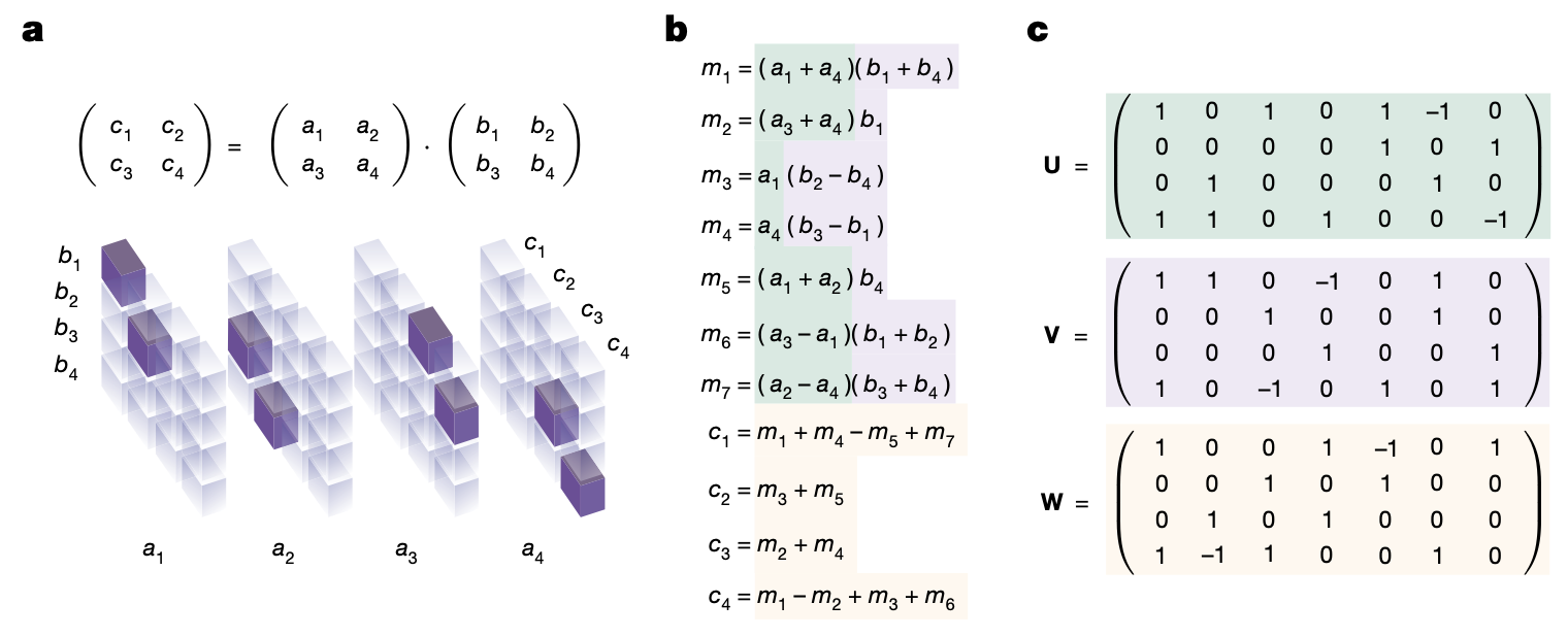
Hence, the optimal matrix multiplication algorithm uses $R = \mathrm{rank}(\mathcal{T}_n)$ multiplications, and decomposition of $\mathcal{T}_n$ into $R$ tensors would give an algorithm. Once we apply the algorithm recursively, it generalizes to a $N \times N$ matrix multiplication algorithm with complexity $O(N^{\log_n R})$. Unfortunately, it is an NP-hard problem to find the rank of a given tensor [4], so it is not easy to find the optimal algorithm. For example, if we try to find a decomposition of $\mathcal{T}_n$ into $R$ vectors of dimension $n$ whose entries are in $\{-1, 0, 1 \}$ (so that the corresponding algorithm does not require additional constant multiplications) in a brute force way, there are $3^{3nR}$ possibilities, which is about $10^{20}$ even for $n =2$ and $R = 7$.

AlphaTensor - how to find a tensor decomposition with reinforcement learning

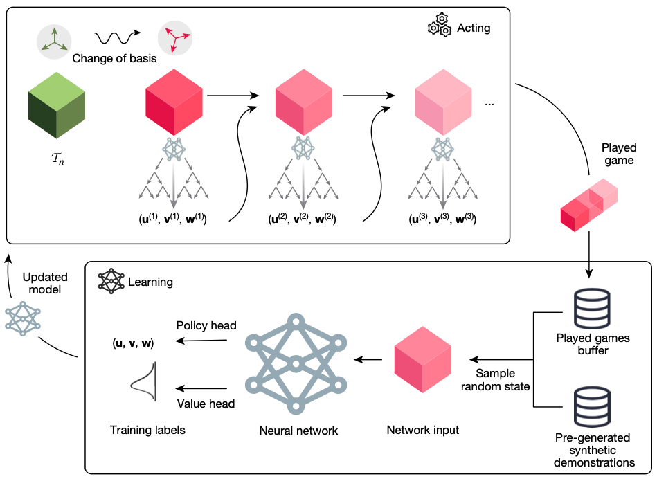
Ok, we’ve reformulated the matrix multiplication as a tensor decomposition problem. How can we solve the tensor decomposition problem, which is NP-hard in general? The author’s idea is to model it as a reinforcement learning problem by a single-player game called TensorGame, and let AI to find the nice decomposition with small number of rank 1 tensors. The below diagram shows the overall flow of TensorGame.

TensorGame

To define a (single-player) game, we need to define state, action, reward, and environment. Each state $\mathcal{S}_t$ is a tensor (of shape $n^2 \times n^2 \times n^2$), and the initial state $\mathcal{S}_0$ is the tensor $\mathcal{T}_n$. At each step, the action is defined as a rank 1 tensor $\mathbf{u}^{(t)} \otimes \mathbf{v}^{(t)} \otimes \mathbf{w}^{(t)}$, and each state is updated by subtracting the rank 1 tensor: $\mathcal{S}_t \leftarrow \mathcal{S}_{t-1} - \mathbf{u}^{(t)} \otimes \mathbf{v}^{(t)} \otimes \mathbf{w}^{(t)}$. Then you may noticed that the goal of the game is to reach the zero tensor $\mathcal{S}_t = \mathbf{0}$ by applying the smallest number of moves, which results a decomposition of $\mathcal{T}_n$ into the sum of rank 1 tensors. To make this work, the authors defined reward as $-1$ for each step to encourage finding shortest path to the zero tensor. Also, they set the limit of the number of steps ($R_{\mathrm{limit}}$) and the agent receives the additional (negative) reward $\gamma(\mathcal{S}_{R_{\mathrm{limit}}})$ when $\mathcal{S}_{R_{\mathrm{limit}}}$ is nonzero, where $\gamma(\mathcal{S}_{R_{\mathrm{limit}}})$ is an upper bound of the rank of the terminal tensor. At last, the entries of $\mathbf{u}^{(t)}, \mathbf{v}^{(t)}, \mathbf{w}^{(t)}$ are constrained as user-specified discrete set of coefficients to find exact multiplication algorithms.

AlphaTensor

AlphaTensor, an agent based on AlphaZero [1], is a player for the TensorGame. It uses Monte Carlo Tree Search (MCTS) algorithm for learning. For each step, based on the output distribution of the policy network, it chooses the action maximizing the probabilistic upper confidence tree bound

\[\underset{a}{\operatorname{argmax}} \,Q(s, a) + c(s) \hat{\pi}(s, a) \frac{\sqrt{\Sigma_b N(s, b)}}{1 + N(s, a)}\]

where

• $N(s, a)$: visit count
• $Q(s, a)$: action value
• $\hat{\pi}(s ,a)$: empirical policy probability
• $c(s)$ exploration factor.

It plays a game until reaches the zero tensor or the limit of the number of steps. Then the game is used to update the parameters of the network.

The following diagram discribes the overall architecture of AlphaTensor, which is composed of torso, policy, and value head.

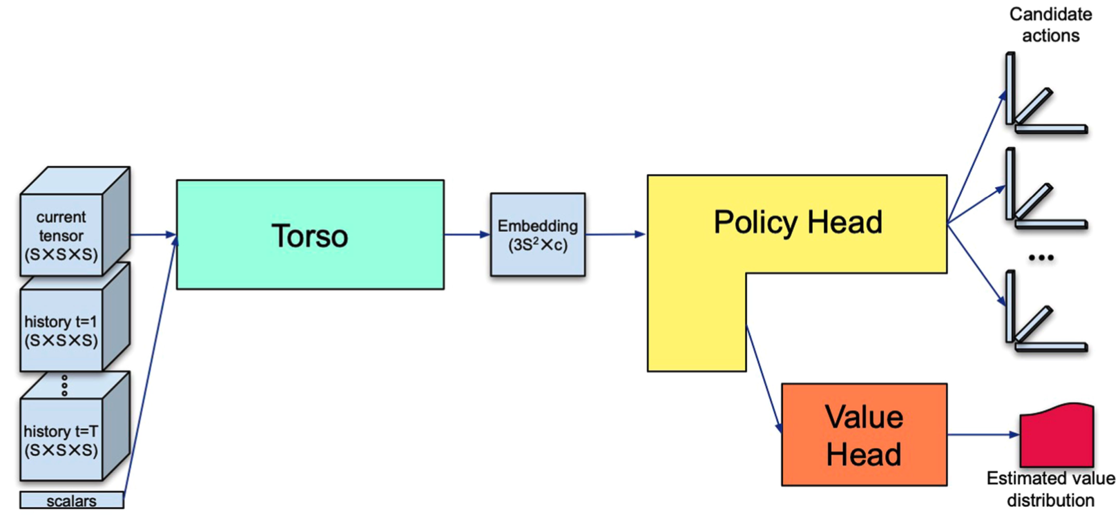
Before I explain the architecture of the network, I’ll describe inputs of the model first. They are composed of a list of tensors and a list of scalars. The list of tensors contain the tensor $\mathcal{S}_t$ of shape $S \times S \times S$ representing the current state, along with the $h$ rank 1 tensors (where $h$ is a hyperparameter, usually set as 7) representing the last $h$ actions, $\mathbf{u}^{(t - 1)}\otimes \mathbf{v}^{(t-1)} \otimes \mathbf{w}^{(t-1)}, \dots, \mathbf{u}^{(t - h)} \otimes \mathbf{v}^{(t -h)}, \otimes \mathbf{w}^{(t - h)}$. The list of scalars includes the time index $t$ of the current action.

The architecture of each of the component are shown in the below diagram.

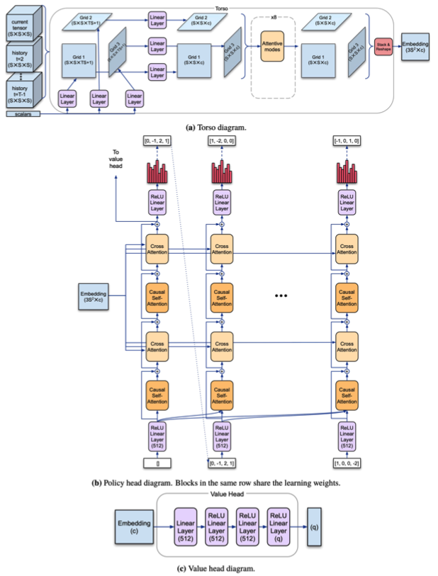
Torso is a network that embeds the input (list of tensors and scalars) as $3S^2$ 512-dimensional vectors, which is based on a modification of transformer architecture. Policy head also uses transformer architecture to model an autoregressive policy. The output of torso is used as input for the cross-attention modules, and the feature representation before the last linear layer is used as an input of the value head. Value head is a 4-layer MLP that produces $q$ outputs corresponding to $\frac{1}{2q}, \frac{3}{2q}, \dots, \frac{2q-1}{2q}$ quantiles, so that it predicts the distribution of returns. At inference time, the average of the predicted values for quantiles over 75% is used to encourage the agent to be risk-seeking.

Synthetic demonstration

Along with the played games, the authors also used simulated games to train the policy network. Although it is hard to decompose a given tensor as a sum of rank 1 tensors, the inverse direction is much easier - we can generate random sequences of rank 1 tensors and add them (although this does not always give the optimal decomposition of the result tensor). This process is used to generate synthetic games and the policy network is trained using these with KL divergence loss. Note that minimizing KL divergence loss maximizes the similarity between the policy and actual action.

Change of basis

Another key step of AlphaTensor is the change of basis. The original tensor $\mathcal{T}_n$ respresents the matrix multiplication in the canonical basis (i.e. the basis composed of the matrices with exactly one 1 and zeros otherwise), and we can represent the matrix multiplication with different basis. More precisely, for given three $S \times S$ invertible matrices $\mathbf{A}, \mathbf{B}, \mathbf{C}$, a tensor $\mathcal{T}$ of shape $S\times S \times S$ transforms into a new tensor $\mathcal{T}^{(\mathbf{A}, \mathbf{B}, \mathbf{C})}$ of the same rank after the change of basis, where the entries of it are

\[\mathcal{T}^{(\mathbf{A}, \mathbf{B}, \mathbf{C})}_{ijk} = \sum_{a=1}^{S} \sum_{b=1}^{S} \sum_{c=1}^{S} \mathbf{A}_{ia} \mathbf{B}_{ib} \mathbf{C}_{ic} \mathcal{T}_{abc}.\]

The authors leverage the observation and use about 100000 different representations of $\mathcal{T}_n$ in terms of different basis and let agent to play the games with different basis in parallel. There are several advantages of using the change of basis:

1. it injects diversity into the games,
2. it exploits properties of the problem as the agent need not succeed in all bases - only need to find a low rank decomposition in any basis,
3. it enlarges the coverage of the algorithm space.

There are some technical restrictions for applying the change of bases. They set $\mathbf{A} = \mathbf{B} = \mathbf{C}$, and also choose matrices of determinant $\pm 1$ so that the inverses also have integer entries (in other words, the matrices are the elements of $\mathrm{GL}_S(\mathbb{Z})$).

Data augmentation

Since changing the order of the rank 1 factors of any decomposition does not change the decomposition itself, we can build additional game sequences from a played game by permuting the orders. The authors used this fact to develop a data augmentation method, by simply swapping a random action with the last action from each finished game.

Results on matrix multiplication algorithms

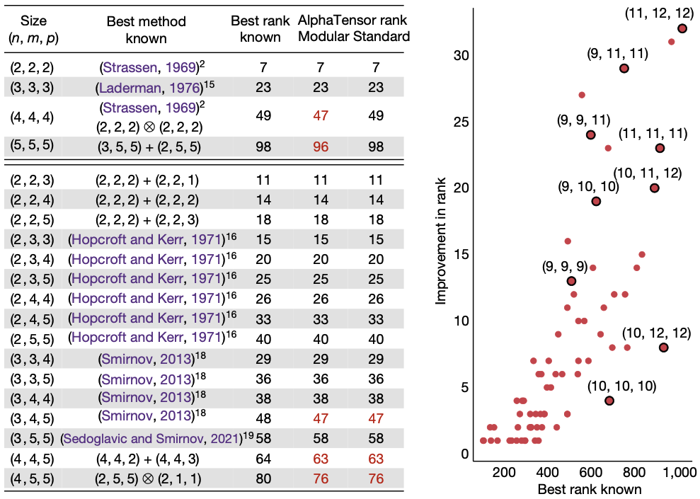
The above table and diagram show the rank of the number of terms in the decomposition of the tensors representing matrix multiplications of certain shapes, which equals to the number of scalar multiplications required for the corresponding matrix multiplication algorithms. As they show, there were improvement in the number of terms for some shapes of tensors compared to the known state of the art decompositions. The last two columns of the table represent decomposition of the same tensor over $\mathbb{Z}_2$ (mod 2 arithmetic) and $\mathbb{R}$ (standard arithmetic), respectively. For example, AlphaTensor found a rank $\leq 47$ decomposition of $\mathcal{T}_4$ that is smaller than the decomposition of the same tensor into $49 = 7^2$ terms that corresponds to Strassen’s two-level algorithm (apply Strassen’s algorithm for 2 by 2 matrices recursively).

Non-standard matrix multiplication

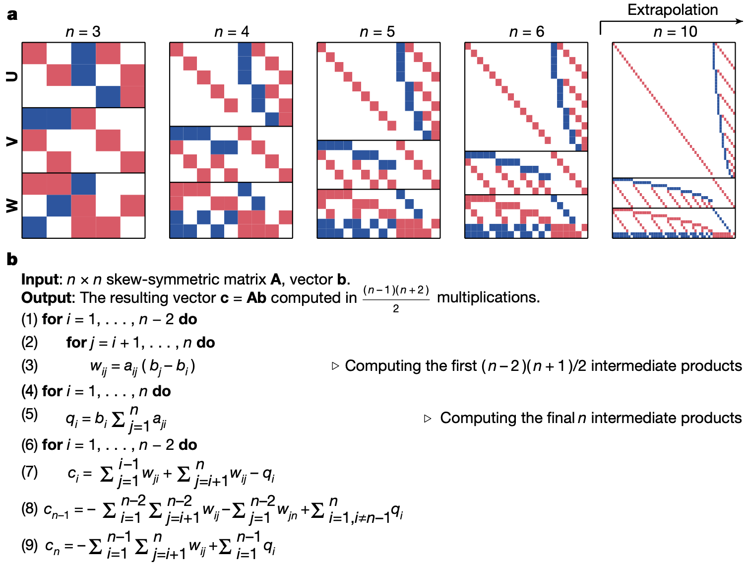
We can also consider a matrix multiplication of structured matrices. For example, the authors tried to decompose a tensor that corresponds to multiplying a $n \times n$ skew-symmetric matrix, i.e. a matrix $A$ satisfying $A^{\intercal} = -A$, with $n$-dimensional vector $v$. Since the space of $n \times n$ skew-symmetric matrices has dimension $\frac{n(n-1)}{2}$ (the matrix is determined by upper diagonal elements), and the bilinear map $(A, v) \mapsto Av$ corresponds to a $\frac{n(n-1)}{2} \times n \times n$ tensor. AlphaTensor found the following decompositions of rank $\frac{(n-1)(n+2)}{2}$ for small $n$’s, and the authors find a pattern and generalize it as an algorithm for any $n$. The corresponding matrix-vector multiplication algorithm uses about $\frac{1}{2}n^2$ multiplications, which is asymptotically twice faster than the known $n^2$ algorithm in [5].

Hardware-aware search

Another interesting point of the AlphaTensor is that it is possible to find hardware-specific tensor decomposition algorithms by modifying a reward function. The authors set a new reward function as

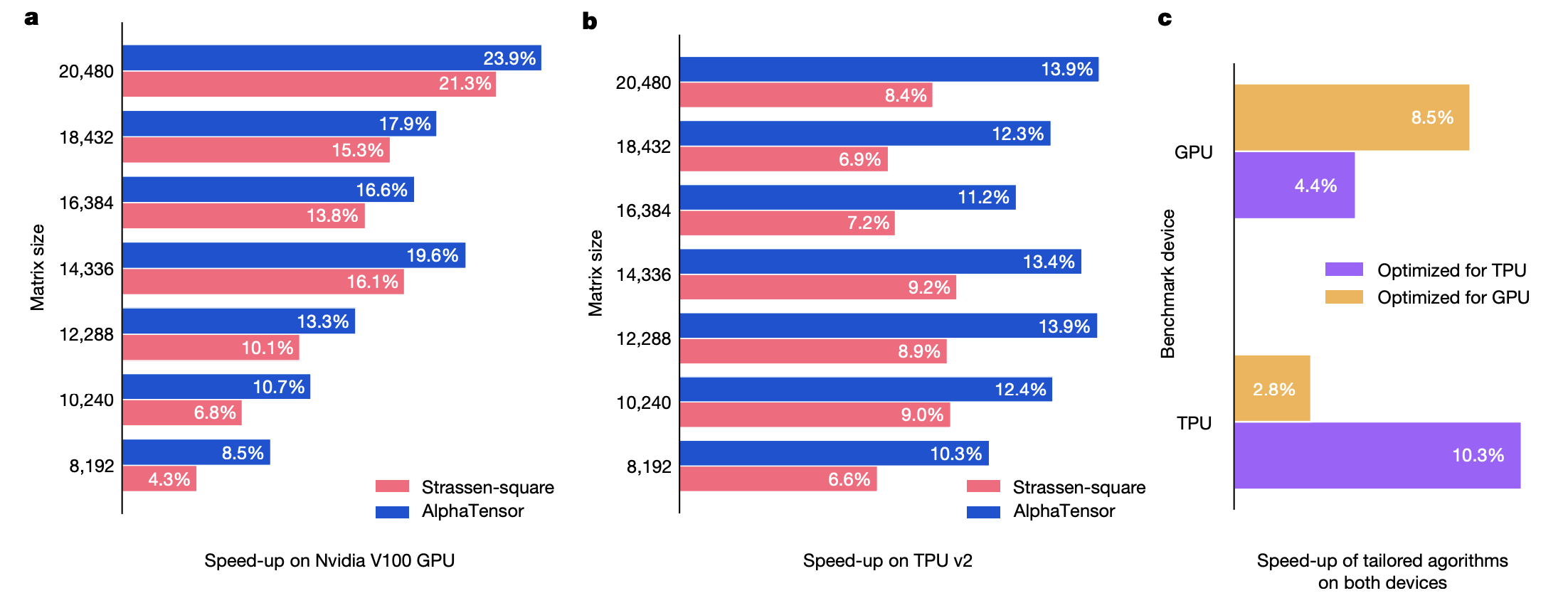
\[r_t' = r_t + \lambda b_t,\]

where $r_t$ is the privous reward for algorithmic discovery, and $b_t$ is a benchmarking reward, the negative of the runtime of the algorithm at the terminal state ($\lambda$ is a hyperparameter). The following graphs show the speed-ups of the algorithms found by AlphaTensor compared to the standard matrix multiplication algorithms (for example, cuBLAS for the GPU) and Strassen-square algorithm for $8192 \times 8192$ matrix multiplications. The figure (c) shows that the algorithm optimized in one hardware do not perform as well on the other hardware, which shows the importance of hardware-aware search.

Conclusion

AlphaTensor shows that it is possible to find practical matrix multiplication algorithms with deep reinforcement learning by reducing the problems as tensor decomposition problems and modeling it as a single-player game called TensorGame. As author mentioned, one may apply the same technique for other problems that can be transformed into tensor decomposition problems, such as a polynomial multiplication. It may even possible to solve other mathematical problems using deep reinforcement learning, and I believe that this is not-too-distant future.

References:

[1] D. Silver et al., Mastering Chess and Shogi by Self-Play with a General Reinforcement Learning Algorithm, preprint (2017)

[2] J. Schrittweiser et al., Mastering Atari, Go, Chess and Shogi by Planning with a Learned Model, Nature (2020)

[3] V. Strassen, Gaussian elimination is not optimal, Numerische Mathematik (1969)

[4] J. Hastad, Tensor Rank is NP-Complete, Journal of Algorithms (1990)

[5] K. Ye, L. Lim, Fast structured matrix computations: tensor rank and Cohn–Umans method, Foundations of Computational Mathematics (2018)

Tags: math  machine-learning