Understanding Astra's result on high-dimensional sphere packing — Part 1: Digestion

The goal of this post is to digest Astra’s proof of the exact asymptotic rate of the optimal Cohn-Elkies linear program and the sign-uncertainty constant. The proof appears in Chapter 1 of OpenAI’s report. The main results are the following:

Theorem 1.1.

\[\lim_{d \to \infty} \mathrm{LP}_{d}^{1/d} = \sqrt{\frac{e}{2\pi}}.\]

In particular,

\[\Delta_d \le 2^{-(\frac{1}{2}\log_2(2\pi/e) + o(1))d} = 2^{-(0.6044\ldots + o(1)) d}.\]

Theorem 1.2.

\[\lim_{d \to \infty} \frac{\mathsf{A}_{+}(d)}{\sqrt{d}} = \lim_{d \to \infty} \frac{\mathsf{A}_{-}(d)}{\sqrt{d}} = \frac{1}{\pi}.\]

I have mostly focused on understanding the intuition behind the proof and making it more readable. Some theorem and lemma statements are rephrased for clarity. Some proofs are expanded with more details, while others are shortened when they are less central to the main ideas.

Problem setting and background

The sphere-packing problem is a very well-known problem in discrete geometry. It asks for the densest packing of congruent spheres in $\mathbb{R}^d$. We denote the optimal packing density by $\Delta_d$. $d = 1$ is trivial ($\Delta_1 = 1$), while the $d = 2$ case was solved by L. Fejes Tóth in the 1940s: the hexagonal ($A_2$-lattice) packing is optimal. The $d = 3$ case is the famous Kepler conjecture, which T. Hales proved in 1998 and the Flyspeck project later formally verified using HOL Light and Isabelle. Viazovska solved the $d = 8$ case in 2016, and Cohn, Kumar, Miller, Radchenko, and Viazovska solved the $d = 24$ case one week later, using the Cohn-Elkies linear-programming (LP) bound introduced below. The other dimensions are still open.

One may ask for bounds in high dimensions. Kabatiansky and Levenshtein (1978) proved the following upper bound:

\[\Delta_d \le 2^{-(0.5990\ldots + o(1)) d}\]

as $d \to \infty$.

The exponent $0.5990\ldots$ remained unchanged, but the multiplicative constant was sharpened: Cohn and Zhao (2014) obtained a multiplier whose geometric average over dimensions is $1/1.2635\ldots$, Sardari and Zargar (2024) obtained $0.4325+51/d$ for $d\ge2000$, and Zargar (2024) later obtained $(1+o(1))/e$. These refinements improve the prefactor, not the exponential rate $2^{-(0.5990\ldots+o(1))d}$.

The sphere-packing problem is closely related to the following optimization problem. We work with “nice” $\mathbb{R}$-valued functions $f$ on $\mathbb{R}^d$, mostly Schwartz functions (denoted by $\mathcal{S}(\mathbb{R}^d;\mathbb{R})$), with Fourier transform

\[\widehat{f}(\xi) = \int_{\mathbb{R}^d} f(x) e^{-2\pi i x \cdot \xi} dx.\]

Let

\[v_d = \frac{\pi^{d/2}}{\Gamma(d/2 + 1)}\]

be the volume of the unit ball in $\mathbb{R}^d$. Consider the set of functions

\[\mathcal{A}_d := \{f \in \mathcal{S}(\mathbb{R}^d;\mathbb{R}) : \widehat{f}(0) > 0, \quad \widehat{f} \ge 0 \,\,\text{on}\,\,\mathbb{R}^d, \quad f(x) \le 0 \,\,\text{on}\,\, |x| \ge 1\}\]

and the associated linear-programming bound

\[\mathrm{LP}_d := \frac{v_d}{2^d} \inf_{f \in \mathcal{A}_d} \frac{f(0)}{\widehat{f}(0)}.\]

The Cohn-Elkies theorem states that the optimal sphere-packing density $\Delta_d$ in $\mathbb{R}^d$ is bounded by

\[\Delta_d \le \mathrm{LP}_d.\]

The proof is based on the Poisson summation formula and is conceptually simple, but the resulting bound is remarkably powerful. It was used to prove the optimality of the $E_8$ and Leech lattices in dimensions 8 and 24: Viazovska and then Cohn, Kumar, Miller, Radchenko, and Viazovska constructed “magic” functions $f$ in $\mathcal{A}_d$ using modular forms that match the densities of those lattice packings. It is also known that the LP bound is suboptimal in dimensions $3,4,5$, by Li, and in dimension $6$, by de Courcy-Ireland, Dostert, and Viazovska.

Cohn and Zhao showed that the LP bound is at least as strong as the KL bound. Later, Afkhami-Jeddi, Cohn, Hartman, de Laat, and Tajdini conjectured that the optimal asymptotic exponent obtainable from the LP bound is better than the KL exponent. More precisely, Conjecture 3.2 in their paper predicts that

\[\lim_{d \to \infty} \mathrm{LP}_d^{1/d} = \sqrt{\frac{e}{2\pi}},\]

which implies

\[\Delta_d \le 2^{-(\frac{1}{2}\log_2(2\pi/e) + o(1))d} = 2^{-(0.6044\ldots + o(1)) d}.\]

They conjectured the constant from numerical experiments, observing that their numerical exponent $0.6044\ldots$ is close to $\log_2(\sqrt{2\pi/e})$. It is remarkable that four decimal digits were enough to suggest the exact expression.

Note that the upper bound is quite far from the best known lower bound. Rogers proved $\Delta_d\ge cd\,2^{-d}$ for sufficiently large $d$, and Venkatesh (2013) improved this by a factor $\log\log d$ along an infinite sequence of dimensions, proving $\Delta_d\ge(1/2-o(1))d\log\log d\,2^{-d}$ there. Campos, Jenssen, Michelen, and Sahasrabudhe (2023) later established the general bound $\Delta_d\ge(1/2-o(1))d\log d\,2^{-d}$ in every sufficiently large dimension. Klartag (2026) then proved the uniform bound $\Delta_d\ge cd^2 2^{-d}$, even for lattice packings; combining Klartag’s method with Venkatesh’s cyclotomic symmetries, Abuya, Gargava, and Zhao (2026) obtained $\Delta_d\ge cd^2\log\log d\,2^{-d}$ along an infinite sequence of dimensions.

The LP bound is also closely related to the Bourgain-Clozel-Kahane sign uncertainty principle. For a Fourier eigenfunction $\widehat g=\varsigma g$, with $\varsigma\in\lbrace-1,+1\rbrace$, define its eventual-nonnegativity radius by

\[r(g):=\inf\{R\ge 0:g(x)\ge0\text{ whenever }|x|\ge R\},\]

and define

\[\mathsf A_{\varsigma}(d):=\inf\{r(g):0\ne g\in L^1(\mathbb R^d;\mathbb R),\ \widehat g=\varsigma g,\ g(0)=0\}.\]

Pointwise values are taken using the continuous representative supplied by Fourier inversion.

It was known that $\mathsf A_+(d)$ and $\mathsf A_-(d)$ are both finite and grow on the order of $\sqrt{d}$. Prior to Astra’s work, the best uniform lower and upper bounds were

\[\sqrt{\frac{d}{4\pi}} \le \mathsf A_+(d) \le \sqrt{\frac{d+2}{2\pi}}\qquad(d\ge5).\]

The upper bound, valid for all $d\ge1$, is by Bourgain-Clozel-Kahane, and the lower bound for $d\ge5$ is by Edwin. Recently, I proved the new upper bound

\[\mathsf A_+(d) \le \sqrt{2\left\lfloor \frac{d}{16}\right\rfloor + 2}\]

for all $d \equiv 0 \pmod{4}$ (prompted by OpenAI’s announcement; see the blog post).

Thoughts on the report

I guess the above introduction is enough to understand the main results (Theorem 1.1 and Theorem 1.2). Here are some comments after reading the report:

• The overall proof is not very long.
• The proof relies heavily on complex analysis.
• The result is asymptotic: it describes what happens as $d\to\infty$. In particular, it does not construct an optimal (or “magic”) function in any specific dimension $d$, which is a much harder problem. The only dimensions in which the exact value of $\mathrm{LP}_d$ is known are $d=1,8,24$. Moreover, knowing $\mathrm{LP}_d$ exactly does not by itself solve sphere packing in dimension $d$, because the LP bound need not be tight: the results cited above prove this in dimensions 3–6, and it is conjectured to be suboptimal in high dimensions as well.
• No modular forms.
• It is easier to understand the proof of the lower bounds than the proof of the upper bounds.
• A previous approach to lower bounds is due to Cohn-Triantafillou. They used a dual formulation of the Cohn-Elkies bound in terms of measures and their Fourier transforms, and constructed examples using modular forms. Astra’s proof takes a different, more elementary and analytic approach: it does not use this dual formulation.
• I still don’t understand how the lower and upper bound exponents match, which seems to be the most interesting point.
• The proof has weird choices of words, such as “Mellin envelope”. I like the proof, but I didn’t enjoy reading the proof.
• One of the core ideas, in my opinion, is to work with the Mellin transform. This idea already appears in Section 5 of the 2016 paper by Cohn and Miller. The report cites CM16 for the radial formulation but does not discuss this particular precedent, which is also mentioned in the recent Scientific American article.
• OpenAI also shared reasoning walkthroughs for the proofs. For the sphere-packing problem, the walkthrough is a sketch or summary rather than Astra’s chain of thought. I first tried reading it before the report, but it wasn’t helpful. It would be more helpful if it were a detailed, raw chain of thought (although these seem to be becoming harder to track these days…).
• I also wonder if Astra would be able to find this proof if the conjectured asymptotic exponent were not given. I think it still might be possible, assuming that it does the numerical experiments itself. However, I do think that knowing about the conjectured decay exponent $\log_2 \sqrt{2\pi/e}$ and the uncertainty principle constant $1/\pi$ might have helped a lot.

Radial and Schwartz reductions

There are some standard reductions that can be made to the problem.

First, one can assume that the functions are radial, i.e., depend only on the norm $\lvert x\rvert$ of $x \in \mathbb{R}^d$, because the linear constraints are rotation-invariant. One can take the average over $\mathrm{O}(d)$ using normalized Haar measure:

\[\mathcal{R}f(x) = \int_{\mathrm{O}(d)} f(Ux) \mathrm{d} U\]

which satisfies

\[\widehat{\mathcal{R}f} = \mathcal{R}\widehat{f}, \quad \mathcal{R}f(0) = f(0), \quad \widehat{\mathcal Rf}(0)=\widehat f(0).\]

This standard argument is also used in constructing magic functions for the $E_8$ and Leech lattices. Radialization also satisfies $r(\mathcal Rg)\le r(g)$, so we may assume that $g$ is radial in the sign uncertainty problem as well.

Second, radial $L^1$ eigenfunctions can be approximated by Schwartz eigenfunctions, which follows from a standard mollification argument. More precisely, suppose that $g \in L^1_{\mathrm{rad}}(\mathbb{R}^d;\mathbb{R})$ satisfies $\widehat{g} = \varsigma g$ and $g(0) = 0$ for some $\varsigma \in \lbrace-1,1\rbrace$. Define

\[g_n = p_n - \frac{p_n(0)}{\psi_{\varsigma}(0)} \psi_{\varsigma}\]

where

\[\begin{align*} &\kappa_n(x) := n^d e^{-\pi n^2|x|^2}, \quad \eta_n(x) := e^{-\pi|x|^2/n^2}, \quad q_n := \eta_n (g * \kappa_n), \\ &p_n := \frac{q_n + \varsigma \widehat{q_n}}{2}, \quad \psi_+(x) := e^{-\pi|x|^2}, \quad \psi_-(x) := \left(|x|^2 - \frac{d}{4\pi}\right) e^{-\pi|x|^2}. \end{align*}\]

Then $g_n \in \mathcal{S}_{\mathrm{rad}}(\mathbb{R}^d;\mathbb{R})$, $\widehat{g}_n = \varsigma g_n$, $g_n(0) = 0$, and $g_n \to g$ in $L^1$ as $n \to \infty$.

Mellin transform

The key idea is to work with the Mellin transform of the radial profile of $g$ rather than directly with $g$. As noted above, this idea already appears in CM16.

We define

\[\lambda = \frac{d}{2}, \quad S_d = \frac{2\pi^{d/2}}{\Gamma(d/2)}\]

where $S_d$ is the surface area of the unit sphere in $\mathbb{R}^d$. For a radial Schwartz function $g$, write $g(r)$ for its one-variable profile. For $\Re z>0$, define

\[M_g(z) = \int_0^{\infty} g(r) r^{z - 1} \mathrm{d}r.\]

On the critical line, set $X_g(t)=M_g(\lambda-it)$. Mellin inversion then gives, for $r>0$,

\[g(r) = \frac{r^{-\lambda}}{2\pi} \int_{\mathbb{R}} X_g(t) r^{it} \,\mathrm dt.\]

The important property of the Mellin transform is that it converts the Fourier transform into simple functional equations. For $0<\Re z<d$, and on the critical line $z=\lambda-it$ with $t\in\mathbb{R}$, respectively, these are

\[M_{\widehat{g}}(z) = \pi^{\lambda - z} \frac{\Gamma(\frac{z}{2})}{\Gamma(\frac{d - z}{2})} M_g(d - z), \quad X_{\widehat{g}}(t) = m_\lambda(t) X_g(-t), \quad m_\lambda(t) = \pi^{it} \frac{\Gamma(\frac{\lambda - it}{2})}{\Gamma(\frac{\lambda + it}{2})}.\]

Lower bound

To prove (asymptotic) lower bounds for $\mathrm{LP}_d$ and $\mathsf A_{\pm}(d)$, one needs a lower bound for the eventual-nonnegativity radius of every relevant function. The key input is the following proposition.

Proposition 3.1. For every $0 < c < 1/\pi$, there exist $C_c, \gamma_c > 0$ and $d_0(c) \in \mathbb{N}$ such that, for every $d \ge d_0(c)$, every $\varsigma \in \lbrace-1,+1\rbrace$, and every nonzero $g \in \mathcal{S}_{\mathrm{rad}}(\mathbb{R}^d;\mathbb{R})$ satisfying $\widehat{g} = \varsigma g$ and $g(0) = 0$, one has

\[\int_{|x| < c \sqrt{d}} |g(x)| \mathrm{d}x \le C_c e^{-\gamma_c d} \|g\|_1.\]

The following proposition is a direct corollary of Proposition 3.1.

Proposition 3.7. For every $0 < c < 1/\pi$, there exists $d_0(c) \in \mathbb{N}$ such that, for every $d \ge d_0(c)$ and every $\varsigma \in \lbrace-1,+1\rbrace$, no nonzero $g \in L^1(\mathbb{R}^d;\mathbb{R})$ satisfies $\widehat{g} = \varsigma g$, $g(0) = 0$, and $g(x) \ge 0$ for $\lVert x\rVert \ge c \sqrt{d}$. Here $g$ denotes its continuous Fourier-inversion representative.

How is this used to prove the lower bounds for $\mathrm{LP}_d$ and $\mathsf A_{\pm}(d)$? Let $F\in\mathcal{A}_d$ be a nonzero function. After rotational averaging, we may assume that $F$ is radial and hence even. Since $\widehat F\ge0$ and $\widehat F(0)>0$, Fourier inversion gives $F(0)=\int\widehat F>0$, so we may set

\[a=\left(\frac{\widehat F(0)}{F(0)}\right)^{1/d}>0,\qquad h(x)=F(ax),\qquad g=\widehat h-h.\]

Indeed,

\[\widehat h(\xi)=a^{-d}\widehat F(\xi/a),\qquad h(0)=\widehat h(0)=F(0).\]

Consequently, $\widehat g=-g$, $g(0)=0$, and the admissibility conditions imply $g(x)\ge0$ for $\lvert x\rvert\ge1/a$. Moreover, $g\ne0$: otherwise $h=\widehat h\ge0$, while $h(x)\le0$ for $\lvert x\rvert\ge1/a$. Thus $h$ would be a nonzero compactly supported self-Fourier function, which is impossible. Proposition 3.7 therefore forces $1/a>c\sqrt d$ for every fixed $c<1/\pi$ and all sufficiently large $d$, and hence

\[\liminf_{d \to \infty} \frac{1}{\sqrt{d}} \inf_{F \in \mathcal{A}_d} \left(\frac{F(0)}{\widehat{F}(0)}\right)^{1/d} \ge c.\]

This holds for every $0 < c < 1/\pi$. Proposition 3.7 gives the same lower bound for each sign-uncertainty radius, namely $\mathsf A_\varsigma(d)\ge c\sqrt d$ for all sufficiently large $d$. Hence

\[\min\left\{\inf_{F \in \mathcal{A}_d} \left(\frac{F(0)}{\widehat{F}(0)}\right)^{1/d}, \mathsf{A}_{-}(d), \mathsf{A}_{+}(d) \right\} \ge \left(\frac{1}{\pi} - o(1)\right) \sqrt{d}.\]

The mysterious constant $\sqrt{e/(2\pi)}$ then comes from

\[v_d^{1/d} = \left(\frac{\pi^{d/2}}{\Gamma(d/2 + 1)}\right)^{1/d} = \sqrt{\frac{2\pi e}{d}} (1 + o(1))\]

and $\sqrt{\frac{e}{2\pi}} = \frac12\sqrt{2\pi e}\cdot\frac1\pi$. The asymptotic formula for $v_d^{1/d}$ follows from Stirling’s formula. In particular, using the definition of $\mathrm{LP}_d$,

\[\liminf_{d\to\infty}\mathrm{LP}_d^{1/d} =\liminf_{d\to\infty}\left[\frac{v_d^{1/d}}{2}\cdot\inf_{F\in\mathcal A_d}\left(\frac{F(0)}{\widehat F(0)}\right)^{1/d}\right] \ge \sqrt{\frac{e}{2\pi}}.\]

We now turn to Proposition 3.1.

Proof overview for Proposition 3.1

The detailed proofs of the intermediate results are collected at the end of this section.

Set $R=c\sqrt d$. We estimate the mass of $g$ inside this ball using the normalized Mellin transform

\[Z(t) = \frac{S_d}{\|g\|_1} R^{\lambda + it} X_g(t).\]

Also consider a normalized version of $g$ in the logarithmic coordinate $r = Re^v$:

\[\varphi(v) = \frac{S_d}{\|g\|_1} (Re^v)^d g(Re^v).\]

This satisfies the following properties:

\[\|\varphi\|_1 = 1, \quad \int_{\mathbb{R}} \varphi(v) \mathrm{d}v = 0, \quad \int_{-\infty}^{0} |\varphi(v)| \mathrm{d}v = \frac{1}{\|g\|_1} \int_{|x| < R} |g(x)| \mathrm{d}x.\]

It is easy to check that these two functions are related by

\[Z(t) = \int_{\mathbb{R}} \varphi(v) e^{-(\lambda + it)v} \mathrm{d}v.\]

The proof of Proposition 3.1 can be divided into the following steps:

1. Bound $Z$ on the strip $\lvert \Im t\rvert\le\lambda$ as $\lvert Z(s + i\sigma\lambda) \rvert \le \exp(H_\sigma(s))$, where $H_\sigma(s)$ can be expressed in terms of the gamma function and the Poisson kernel (Lemma 3.2).
2. Prove that $H_\sigma(s)$ attains its maximum at $s=0$, and estimate $H_\sigma(0)$ in terms of an integral $J_\sigma$ (Lemma 3.3).
3. Evaluate the limit of $J_\sigma$ as $\sigma \to 1^{-}$; this is where the threshold $c<1/\pi$ appears (Lemma 3.4).
4. Combine uniform negativity with a logarithmic tail bound to obtain an exponentially small $L^1$ bound for $Z$ (Lemma 3.5).
5. Apply shifted Mellin/Fourier inversion to transfer the $L^1$ bound for $Z$ to the mass of $\varphi$ over $(-\infty,0)$ (Lemma 3.6).

Let’s start with the first step.

Lemma 3.2. For every $-1 < \sigma < 1$, the function $Z$ is bounded and holomorphic on a neighborhood of the strip $\lvert \Im t\rvert\le\lambda$. Its boundary values satisfy $\lvert Z(y+i\lambda)\rvert\le1$ and $\log\lvert Z(y-i\lambda)\rvert\le h_\lambda(y)$ for $y\ne0$, where the lower-boundary majorant is

\[h_\lambda(y) = \lambda \log(\pi R^2) + \log |\Gamma(-iy/2)| - \log |\Gamma(\lambda + iy/2)|.\]

Writing $\theta = \pi(1+\sigma)/2$, define

\[P_\sigma(T) = \frac{\sin\theta}{4(\cosh(\pi T/2) - \cos\theta)}, \quad M_\sigma = \int_{\mathbb{R}} P_\sigma(T) \mathrm{d}T = \frac{1-\sigma}{2}.\]

Then

\[|Z(s + i\sigma\lambda)| \le \exp(H_\sigma(s)), \quad H_\sigma(s) = \int_{\mathbb{R}} P_\sigma(T) h_\lambda(s - \lambda T) \mathrm{d}T \quad (s \in \mathbb{R}).\]

It is easy to bound $\lvert Z \rvert$ on the upper boundary $\Im t = \lambda$, and the bound for the lower boundary $\Im t = -\lambda$ follows from the functional equation. For the general bound inside the strip, we use a conformal map that sends the strip to the upper half plane, and apply the Poisson inequality there.

Next, we bound $H_\sigma$. Lemma 3.3 and Lemma 3.4 are intermediate steps toward Lemma 3.5.

Lemma 3.3. For every $-1 < \sigma < 1$, there exists $C_\sigma > 0$, independent of $d$, $c$, and $g$, such that

\[\int_{\mathbb{R}} P_\sigma(T) \left|h_\lambda(\lambda T) - \lambda \left(\log(2\pi c^2) - \int_0^1 \log \sqrt{x^2 + T^2/4} \mathrm{d}x\right)\right| \mathrm{d}T \le C_\sigma \log(2 + \lambda).\]

Define

\[J_\sigma := -\frac{1}{M_\sigma} \int_{\mathbb{R}} P_\sigma(T) \int_0^1 \log \sqrt{x^2 + T^2/4} \mathrm{d}x \mathrm{d}T.\]

Then, for every $s \in \mathbb{R}$,

\[H_\sigma(s) \le H_\sigma(0) = \lambda M_\sigma (\log(2\pi c^2) + J_\sigma) + O_\sigma(\log(2 + \lambda)).\]

The error estimate is based on the Riemann sum approximation of $h_\lambda(\lambda T)$.

Now, our goal is to show that $H_\sigma(0)\le-\gamma\lambda$ for some $\gamma>0$, making $e^{H_\sigma(0)}$ exponentially small in $\lambda=d/2$. First, we compute the limit of $J_\sigma$ as $\sigma \to 1^{-}$.

Lemma 3.4. For $J_\sigma$ defined in Lemma 3.3,

\[\lim_{\sigma \to 1^{-}} J_\sigma = \log\frac{\pi}{2}.\]

Consequently, for every $0<c<1/\pi$, there exists $\sigma(c)\in(-1,1)$ such that $\log(2\pi c^2)+J_{\sigma(c)}<0$.

This is precisely where the constant $1/\pi$ enters, since

\[\log(2\pi c^2)+\log(\pi/2)=\log(\pi^2c^2)<0 \quad\Longleftrightarrow\quad c<1/\pi.\]

From now on, fix $\sigma=\sigma(c)$ such that $\log(2\pi c^2)+J_\sigma<0$.

Lemma 3.5. There exist $\gamma_c, C_c^{\prime}, B_c > 0$, depending only on $c$, such that, for every sufficiently large $d$,

\[H_\sigma(s) \le -\gamma_c \lambda \quad(s \in \mathbb{R}), \quad \int_{\mathbb{R}} |Z(s + i\sigma\lambda)| \mathrm{d}s \le C_c' \lambda e^{-\gamma_c \lambda}.\]

Moreover, after increasing $B_c$ if necessary,

\[H_\sigma(\lambda S) \le - \frac{M_\sigma \lambda}{2} \log \frac{|S|}{C_c'} \quad (|S| \ge B_c).\]

Using Lemma 3.5, we can bound the integral of $\lvert \varphi\rvert$ over $(-\infty,0)$.

Lemma 3.6. For every $0 < c < 1/\pi$, there exist $C_c, \gamma_c > 0$ and $d_0(c) \in \mathbb{N}$, independent of $g$ and $\varsigma$, such that, for every $d\ge d_0(c)$,

\[\int_{-\infty}^{0} |\varphi(v)| \mathrm{d}v \le C_c e^{-\gamma_c d}.\]

Proposition 3.1 now follows from the identity

\[\int_{-\infty}^{0}|\varphi(v)|\,\mathrm dv =\frac1{\|g\|_1}\int_{|x|<c\sqrt d}|g(x)|\,\mathrm dx.\]

Proofs of intermediate results

Lemma 3.2

The bounds on the upper and lower boundaries of the strip are just intermediate steps, and the main goal is to bound $Z$ inside the strip. This follows by applying the upper half plane Poisson inequality to $\log\lvert Z\rvert$.

Upper half plane Poisson inequality. Let $b : \mathbb{R} \to \mathbb{R}$ satisfy the weighted integrability needed below, and define $P[b] : \mathbb{H} \to \mathbb{R}$ by

\[P[b](x + iy) = \frac{1}{\pi} \int_{\mathbb{R}} \frac{y}{(t - x)^2 + y^2} b(t) \mathrm{d}t.\]

If $u$ is subharmonic and bounded above on $\mathbb H$, and its boundary values on $\mathbb R = \partial\mathbb H$ are bounded above by $b$, then $u\le P[b]$ on $\mathbb H$.

We have $g(r),\widehat g(r)=O(r^2)$ at the origin. The Mellin transforms therefore continue past $\operatorname{Re}z=0$, and $Z$ is holomorphic on a neighborhood of the closed strip. On its upper boundary,

\[Z(y+i\lambda)=\int_{\mathbb R}\varphi(v)e^{-iyv}\,\mathrm{d}v, \qquad |Z(y+i\lambda)|\le\|\varphi\|_1=1.\]

The Mellin functional equation gives the lower-boundary identity

\[Z(y-i\lambda) = \varsigma (\pi R^2)^{\lambda + iy} \frac{\Gamma(-iy/2)}{\Gamma(\lambda + iy/2)} Z(-y + i\lambda).\]

Taking absolute values proves the claimed lower-boundary estimate for $y\ne0$. At $y=0$, the zero $Z(i\lambda)=\int\varphi=0$ cancels the apparent pole of $\Gamma(-iy/2)$, so $Z$ remains bounded there. More generally, for $-\lambda\le\eta\le\lambda$,

\[|Z(s+i\eta)| \le \frac{S_dR^{\lambda-\eta}}{\|g\|_1} \int_0^\infty |g(r)|r^{\lambda+\eta-1}\,\mathrm{d}r.\]

Splitting the integral at $r=1$, using $g(r)=O(r^2)$ near zero and rapid decay at infinity, makes this bound uniform in $s$ and $\eta$. Thus $Z$ is bounded on the whole closed strip.

To prove the interior bound, map the strip to the upper half plane and invoke the Poisson inequality there. The conformal map is

\[\Phi(z) = \exp\left(\frac{\pi(z + i\lambda)}{2\lambda}\right)\]

which maps the lower boundary $\Im z=-\lambda$ to $(0,\infty)$ and the upper boundary $\Im z=\lambda$ to $(-\infty,0)$. It maps $z=s+i\sigma\lambda$ to

\[\Phi(s + i\sigma\lambda) = \rho e^{i\theta}, \quad \rho = \exp\left(\frac{\pi s}{2\lambda}\right), \quad \theta = \frac{\pi(1+\sigma)}{2}.\]

The map is a biholomorphism from the strip $\lvert \Im z\rvert<\lambda$ to the upper half-plane $\mathbb{H}$. Since $Z\circ\Phi^{-1}$ is holomorphic, $u(z)=\log\lvert Z(\Phi^{-1}(z))\rvert$ is subharmonic, with the value $-\infty$ allowed at its zeros. One technical difficulty is that $h_\lambda(y)$ has a singularity at $y=0$:

\[h_\lambda(y) = -\log|y| + O_\lambda(1),\quad y \to 0.\]

To deal with this, truncate $h_\lambda$. As mentioned above, $Z$ is bounded on the closed strip, hence on the lower boundary. So we can truncate $h_\lambda$ to a function $h_{\lambda,D}$ that is bounded above:

\[h_{\lambda,D}(y)= \begin{cases} \min\{h_\lambda(y),D\},&y\ne0,\\ D,&y=0. \end{cases}\]

and choose $D>\max\lbrace0,\sup_{y \in \mathbb{R}}\log\lvert Z(y-i\lambda)\rvert\rbrace$. Since $\log\lvert Z\rvert\le0$ on the upper boundary, which maps to the negative real axis under $\Phi$, we may majorize its boundary data there by zero and only integrate the nontrivial data over the positive real axis:

\[\begin{align*} \log |Z(s + i\sigma \lambda)| &= u(\Phi(s + i\sigma\lambda)) \\ &\le \int_{0}^{\infty} \frac{1}{\pi} \cdot \frac{\rho\sin\theta}{(t - \rho\cos\theta)^2 + (\rho\sin\theta)^2} h_{\lambda, D}\!\left(\frac{2\lambda}{\pi}\log t\right) \mathrm{d}t, \end{align*}\]

where $\Phi(s+i\sigma\lambda)=\rho\cos\theta+i\rho\sin\theta$. Now substitute $t=e^{\pi y/(2\lambda)}$, corresponding to the lower-boundary point $y-i\lambda$. Since

\[\mathrm{d}t=\frac{\pi t}{2\lambda}\,\mathrm{d}y, \qquad (t-\rho\cos\theta)^2+(\rho\sin\theta)^2 =t^2-2\rho t\cos\theta+\rho^2,\]

the usual upper-half-plane Poisson measure becomes

\[\begin{aligned} \frac{1}{\pi} \frac{\rho\sin\theta} {(t-\rho\cos\theta)^2+(\rho\sin\theta)^2}\,\mathrm{d}t &= \frac{\sin\theta}{2\lambda} \frac{\rho t}{t^2-2\rho t\cos\theta+\rho^2}\,\mathrm{d}y\\ &= \frac{\sin\theta}{2\lambda\left(t/\rho+\rho/t-2\cos\theta\right)}\,\mathrm{d}y \\ &= \frac{\sin\theta} {4\lambda\left(\cosh\left(\frac{\pi(s-y)}{2\lambda}\right)-\cos\theta\right)}\,\mathrm{d}y \\ &= \frac{1}{\lambda} P_\sigma\left(\frac{s-y}{\lambda}\right)\,\mathrm{d}y. \end{aligned}\]

Substituting this identity into the Poisson integral gives

\[\begin{align*} \int_{0}^{\infty} \frac{1}{\pi} \cdot \frac{\rho\sin\theta}{(t - \rho\cos\theta)^2 + (\rho\sin\theta)^2} h_{\lambda, D}\!\left(\frac{2\lambda}{\pi}\log t\right) \mathrm{d}t &= \int_{\mathbb{R}} \frac{1}{\lambda} P_\sigma\left(\frac{s-y}{\lambda}\right) h_{\lambda, D}(y) \mathrm{d}y \\ &= \int_{\mathbb{R}} P_\sigma(T) h_{\lambda, D}(s - \lambda T) \mathrm{d}T. \end{align*}\]

The logarithmic singularity of $h_\lambda$ is locally integrable, and the exponential decay of $P_\sigma$ controls its logarithmic growth in absolute value at infinity. Dominated convergence therefore permits $D\to\infty$ and proves $\log\lvert Z(s+i\sigma\lambda)\rvert\le H_\sigma(s)$. $\square$

Lemma 3.3

We have

\[H_\sigma(0) = \int_{\mathbb{R}} P_\sigma(T) h_\lambda(-\lambda T) \mathrm{d}T = \int_{\mathbb{R}} P_\sigma(T) h_\lambda(\lambda T) \mathrm{d}T,\]

since $P_\sigma$ and $h_\lambda$ are even functions. Thus the first estimate implies

\[\lvert H_\sigma(0) - \lambda M_\sigma (\log(2\pi c^2) + J_\sigma)\rvert \le C_\sigma \log(2 + \lambda).\]

This is the final estimate in the lemma. We will focus on proving this estimate and $H_\sigma(s) \le H_\sigma(0)$. The following elementary lemma is used in the last step of the proof and is worth mentioning.

Lemma (Convolution of even nonnegative monotone functions). Let $f$ and $g$ be nonnegative integrable even functions on $\mathbb{R}$ that are decreasing on $[0,\infty)$. Then their convolution $f * g$ is maximized at $0$.

Proof. We have

\[f(x) = \int_0^\infty \mathbf{1}_{\{f(x) > a\}} \,\mathrm{d}a, \qquad g(x) = \int_0^\infty \mathbf{1}_{\{g(x) > b\}} \,\mathrm{d}b.\]

Up to endpoints, write

\[(-r_a, r_a) = \{f(x) > a\}, \qquad (-R_b, R_b) = \{g(x) > b\}.\]

Then Tonelli’s theorem gives

\[(f * g)(x) = \int_{0}^{\infty} \int_{0}^{\infty} \lvert(-R_b, R_b) \cap (x - r_a, x + r_a)\rvert \,\mathrm{d}a\,\mathrm{d}b,\]

and the length of the intersection is maximized at $x=0$. $\square$

Proof of Lemma 3.3. The difference between $h_\lambda(\lambda T)$ and

\[\lambda\left(\log(2\pi c^2) - \int_0^1 \log \sqrt{x^2 + \frac{T^2}{4}} \mathrm{d}x\right)\]

is bounded by expressing $h_\lambda(\lambda T)$ in terms of Riemann sums of $f_T(x)=\log\sqrt{x^2+T^2/4}$ and controlling the error. For example, if $d=2n$ is even, then $n=\lambda$. For $T\ne0$, the identities $\Gamma(z+1)=z\Gamma(z)$ and $\lvert \Gamma(ib)\rvert=\lvert \Gamma(-ib)\rvert$ for $b \in \mathbb{R}$ give

\[h_n(nT) = n\log(2\pi c^2) - \sum_{k=0}^{n-1} f_T\left(\frac{k}{n}\right)\]

and monotonicity of $f_T$ gives

\[0 \le h_n(nT) - n \left(\log(2\pi c^2) - \int_0^1 f_T(x) \mathrm{d}x \right) \le f_T(1) - f_T(0) = \frac{1}{2} \log \left(1 + \frac{4}{T^2}\right).\]

Multiplying this bound by the Poisson kernel $P_\sigma(T)$ gives an integrable function. Near $T=0$, the bound is $O(1+\log(1/\lvert T\rvert))$, which is locally integrable; for $\lvert T\rvert>1$, it is $O(T^{-2})$, while $P_\sigma$ decays exponentially. Its integral is therefore bounded by a constant depending only on $\sigma$, not on $n$, $c$, or $g$.

When $d=2n+1$ is odd, so that $\lambda=n+\tfrac12$, set $b=\lambda T/2$ and use the identity

\[\frac{\lvert\Gamma(-ib)\rvert^2} {\lvert\Gamma(\frac12+ib)\rvert^2} =\frac{\coth(\pi\lvert b\rvert)}{\lvert b\rvert}\]

to obtain

\[h_\lambda(\lambda T) =\lambda\log(2\pi c^2) -\sum_{k=0}^{n-1}f_T\left(\frac{k+1/2}{\lambda}\right) +\frac12\log\lambda +\frac12\log\frac{\coth(\pi \lambda \lvert T\rvert /2)}{\lambda\lvert T\rvert/2}.\]

In this case, split

\[\int_0^1 f_T(x)\,\mathrm{d}x =\int_0^{n/\lambda}f_T(x)\,\mathrm{d}x +\int_{n/\lambda}^1f_T(x)\,\mathrm{d}x,\]

and compare the first integral with the midpoint sum:

\[\begin{aligned} &h_\lambda(\lambda T) -\lambda\left(\log(2\pi c^2)-\int_0^1f_T(x)\,\mathrm{d}x\right)\\ &=\lambda \left(\int_0^{\frac{n}{\lambda}} f_T(x)\,\mathrm{d}x -\frac{1}{\lambda}\sum_{k=0}^{n-1}f_T\left(\frac{k+1/2}{\lambda}\right) \right) +\lambda\int_{\frac{n}{\lambda}}^1f_T(x)\,\mathrm{d}x \\ &\quad +\frac12\log\lambda + \frac12\log\frac{\coth(\pi \lambda \lvert T\rvert /2)}{\lambda\lvert T\rvert/2}. \end{aligned}\]

By monotonicity, the first term on the right, including its prefactor $\lambda$, has absolute value at most

\[f_T(n/\lambda)-f_T(0) \le f_T(1)-f_T(0) =\frac12\log\left(1+\frac4{T^2}\right).\]

The remaining interval has length $1/(2\lambda)$. Together, these two contributions are bounded by

\[C\left(1+\log(2+|T|)+\log(2+|T|^{-1})\right).\]

The endpoint correction is controlled by the same $T$-dependent logarithms, together with an additional $C\log(2+\lambda)$. Thus the total error is bounded by

\[C\left(1 + \log(2 + \lvert T \rvert) + \log (2 + \lvert T \rvert^{-1}) + \log(2 + \lambda)\right),\]

and integrating against $P_\sigma(T)\,\mathrm{d}T$ gives the desired bound, with a constant depending on $\sigma$.

It remains to prove that $H_\sigma(s)$ is maximized at $s=0$. Since $P_\sigma$ and $h_\lambda$ are even, $H_\sigma$ is even. It is clear that $P_\sigma(T)$ is decreasing on $(0, \infty)$, and $h_\lambda(y)$ is also decreasing for $y>0$, since

\[h_\lambda'(y) = \frac{\Im\psi(\lambda + iy/2) - \Im\psi(iy/2)}{2} < 0,\]

for $y > 0$, where $\psi = \Gamma^{\prime}/\Gamma$ is the digamma function and $\Im\psi(a + bi) = \sum_{k \ge 0} \frac{b}{(k+a)^2 + b^2}$. Consider $q_{\lambda, N}(u) := \max\lbrace h_\lambda(\lambda u) + N, 0\rbrace$. It is nonnegative, even, and decreasing on $(0,\infty)$; it is also integrable because the singularity at zero is logarithmic and $h_\lambda(y)\to-\infty$ as $|y|\to\infty$. The convolution lemma therefore gives

\[(P_\sigma*q_{\lambda,N})(s/\lambda) \le (P_\sigma*q_{\lambda,N})(0).\]

Subtracting the constant $NM_\sigma$ and using $q_{\lambda,N}(u)-N=\max\lbrace h_\lambda(\lambda u),-N\rbrace$ turns this into

\[\int_{\mathbb{R}} P_\sigma(T) \max\lbrace h_\lambda(s-\lambda T),-N\rbrace\,\mathrm{d}T \le \int_{\mathbb{R}} P_\sigma(T) \max\lbrace h_\lambda(-\lambda T),-N\rbrace\,\mathrm{d}T.\]

The exponential decay of $P_\sigma$ controls the logarithmic behavior of $h_\lambda$, so passing to the limit $N \to \infty$ gives $H_\sigma(s) \le H_\sigma(0)$. $\square$

Lemma 3.4

After making the substitution $T=2u$ and normalizing by the mass $M_\sigma$, we get

\[p_\sigma(u)=\frac{2P_\sigma(2u)}{M_\sigma} =\frac{\sin\theta}{(1-\sigma)(\cosh(\pi u)-\cos\theta)}.\]

As $\sigma\to1^{-}$, these densities converge in $L^1$ to

\[p(u)=\frac\pi4\operatorname{sech}^2\left(\frac{\pi u}{2}\right).\]

Its characteristic function is

\[\int_{\mathbb{R}} p(u) e^{itu} \mathrm{d}u = \frac{t}{\sinh t}.\]

Define

\[I(x)=\int_{\mathbb R}p(u)\log\sqrt{x^2+u^2}\,\mathrm{d}u.\]

Then the Laplace representation of $x/(x^2+u^2)$ gives, for $x>0$,

\[I'(x)=\int_0^\infty e^{-xt}\frac{t}{\sinh t}\,\mathrm{d}t =\frac12\psi'\left(\frac{x+1}{2}\right),\]

where $\psi = \Gamma^{\prime}/\Gamma$ is the digamma function. Matching the constants from the common asymptotic $\log x+o(1)$ as $x\to\infty$ therefore gives

\[\int_{\mathbb R}p(u)\log\sqrt{x^2+u^2}\,\mathrm{d}u =\psi\left(\frac{x+1}{2}\right)+\log2.\]

Local integrability of $\log\lvert u\rvert$ extends this identity to $x=0$. The uniform exponential bound $p_\sigma(u)\ll e^{-\pi\lvert u\rvert}$ then justifies dominated convergence in $J_\sigma$. Finally,

\[\int_0^1\psi\left(\frac{x+1}{2}\right)\,\mathrm{d}x =2\log\frac{\Gamma(1)}{\Gamma(1/2)}=-\log\pi,\]

and integrating the preceding identity over $0\le x\le1$ yields $\lim_{\sigma\to1^-}J_\sigma=\log(\pi/2)$. $\square$

Lemma 3.5

Set

\[\delta_c=-\bigl(\log(2\pi c^2)+J_\sigma\bigr)>0.\]

Lemma 3.3 gives

\[H_\sigma(s)\le-\lambda M_\sigma\delta_c+O_\sigma(\log\lambda) \le-\gamma_c\lambda,\]

for every $s$ once $d$ is sufficiently large. The resulting constant upper bound $e^{-\gamma_c\lambda}$ for $e^{H_\sigma(s)}$ is not integrable over $\mathbb{R}$, so we also need a tail estimate (i.e., a bound for large $\lvert s \rvert$). The gamma-function identities give, for $U\ne0$,

\[h_\lambda(\lambda U) \le \lambda\log\frac{4\pi c^2}{|U|}+E_\lambda(U),\]

because every gamma-recurrence factor has modulus at least $\lvert \lambda U\rvert/2$; in odd dimensions, the remaining half-integer ratio contributes the error $E_\lambda(U)$. Here

\[E_\lambda(U)= \begin{cases} 0,&\lambda\in\mathbb N,\\ \dfrac12\log\coth\left(\dfrac{\pi\lambda|U|}{2}\right), &\lambda\in\mathbb N+\dfrac12. \end{cases}\]

In the odd-dimensional case,

\[\int_{\mathbb R}E_\lambda(U)\,\mathrm{d}U =\frac{2}{\pi\lambda}\int_0^\infty\log\coth x\,\mathrm{d}x =\frac{\pi}{4\lambda}.\]

Hence the $P_\sigma$-convolution of $E_\lambda$ is $O_\sigma(\lambda^{-1})$ in both parities, and

\[H_\sigma(\lambda S) \le \lambda M_\sigma\log(4\pi c^2) -\lambda\int_{\mathbb R}P_\sigma(T)\log|S-T|\,\mathrm{d}T +O_\sigma(\lambda^{-1}).\]

Split the logarithmic integral at $\lvert T\rvert =\lvert S\rvert /2$. On the inner part, $\lvert S-T\rvert \ge \lvert S\rvert /2$ and the omitted $P_\sigma$-mass is exponentially small. On the outer part, the only possible negative contribution occurs near $T=S$; exponential decay of $P_\sigma(T)$ and local integrability of $\log \lvert S-T\rvert$ control it. Thus there are $B_c,A_c>0$ such that

\[\int_{\mathbb R}P_\sigma(T)\log|S-T|\,\mathrm{d}T \ge\frac{M_\sigma}{2}\log|S|-A_c \qquad(|S|\ge B_c),\]

which yields the stated logarithmic tail bound after enlarging $C_c^{\prime}$ if necessary.

Finally, choose $B>\max\lbrace B_c,C_c^{\prime}\rbrace$ and put $q=M_\sigma\lambda/2>1$. On the central interval, uniform negativity gives

\[\int_{|s|\le B\lambda}e^{H_\sigma(s)}\,\mathrm{d}s \le2B\lambda e^{-\gamma_c\lambda}.\]

On its complement, substitute $s=\lambda S$ and use the logarithmic tail:

\[\int_{|s|>B\lambda}e^{H_\sigma(s)}\,\mathrm{d}s \le\frac{2\lambda C_c'}{q-1} \left(\frac{B}{C_c'}\right)^{1-q}.\]

The second expression also decays exponentially in $\lambda$. After decreasing $\gamma_c$ and enlarging the constant, Lemma 3.2 gives

\[\int_{\mathbb R}|Z(s+i\sigma\lambda)|\,\mathrm{d}s \le C_c'\lambda e^{-\gamma_c\lambda}.\]

This proves the lemma. $\square$

Lemma 3.6

Set $G(v)=e^{(\sigma-1)\lambda v}\varphi(v)$. The required integrability follows directly from

\[\int_{\mathbb R}|G(v)|\,\mathrm{d}v =\frac{S_dR^{(1-\sigma)\lambda}}{\|g\|_1} \int_0^\infty|g(r)|r^{(1+\sigma)\lambda-1}\,\mathrm{d}r <\infty.\]

Its Fourier transform $\int_{\mathbb R}G(v)e^{-isv}\,\mathrm{d}v$ is $Z(s+i\sigma\lambda)$. Lemma 3.5 makes this transform integrable, so Fourier inversion gives

\[\varphi(v) = \frac{e^{(1 - \sigma)\lambda v}}{2\pi} \int_{\mathbb{R}} Z(s + i\sigma\lambda) e^{isv} \mathrm{d}s.\]

Taking absolute values and integrating over $v \in (-\infty, 0)$, we get

\[\begin{align*} \int_{-\infty}^{0} |\varphi(v)| \mathrm{d}v &\le \frac{1}{2\pi} \int_{-\infty}^{0} e^{(1 - \sigma)\lambda v} \mathrm{d}v \int_{\mathbb{R}} |Z(s + i\sigma\lambda)| \mathrm{d}s \\ &= \frac{1}{2\pi (1 - \sigma)\lambda} \int_{\mathbb{R}} |Z(s + i\sigma\lambda)| \mathrm{d}s \le \frac{C_c'}{2\pi(1-\sigma)}e^{-\gamma_c d/2}, \end{align*}\]

where $\lambda=d/2$. Absorbing $C_c^{\prime}/(2\pi(1-\sigma))$ and the factor $1/2$ in the exponent into new positive constants gives the asserted form $C_ce^{-\gamma_cd}$. $\square$

Proposition 3.7

If $g$ is a radial Schwartz function, then $\int g = \widehat{g}(0) = \varsigma g(0) = 0$, and hence its negative part $g_- = \max\lbrace-g,0\rbrace$ has integral $\lVert g\rVert_1/2$. If $g(x) \ge 0$ for $\lVert x\rVert \ge c \sqrt{d}$, then $g_-$ vanishes outside the ball of radius $c \sqrt{d}$ and

\[\frac{\|g\|_{1}}{2} = \int_{\mathbb{R}^d} g_{-}(x) \mathrm{d}x = \int_{|x| < c \sqrt{d}} g_{-}(x) \mathrm{d}x \le \int_{|x| < c \sqrt{d}} |g(x)| \mathrm{d}x \le C_c e^{-\gamma_c d} \|g\|_1.\]

This is a contradiction for large $d$.

For a general $g\in L^1$, first replace it by its radialization $h=\mathcal Rg$. This radialization is still nonzero: if $h=0$, then outside a ball the function $g$ is nonnegative with zero spherical average, so it vanishes there. The identity $\widehat g=\varsigma g$ and Fourier analyticity would then force $g=0$. Let $h_n$ be the radial Schwartz eigenfunctions constructed above. They need not remain nonnegative outside the ball, but $(h_n)_-\le \lvert h_n-h \rvert$ outside the ball. Thus, with $R=c\sqrt d$,

\[\frac12\|h_n\|_1=\int_{\mathbb R^d}(h_n(x))_-\,\mathrm{d}x \le \int_{|x|<R}|h_n(x)|\,\mathrm{d}x+\|h_n-h\|_1.\]

Proposition 3.1 bounds the first term. Letting $n\to\infty$ gives $\lVert h\rVert_1/2\le C_ce^{-\gamma_cd}\lVert h\rVert_1$, again a contradiction for large $d$. $\square$

Upper bound

To prove the upper bounds, one needs to construct asymptotically optimal functions. The report does not construct exact optimizers in any dimension, which is much harder.

For each sufficiently small fixed $\epsilon>0$ and all sufficiently large $d$, the proof constructs radial Schwartz functions $f_-$, $f_+$, and $f_0$, together with a radius $R_{\epsilon,d}$, such that

\[\widehat f_-=f_+>0,\qquad \widehat f_0=f_0,\qquad f_-(0)=f_+(0)>0,\qquad f_0(0)=0,\]

and

\[f_-(x)<0<f_0(x)\qquad(|x|\ge R_{\epsilon,d}).\]

Moreover,

\[\lim_{\epsilon\to 0^+}\lim_{d\to\infty}\frac{R_{\epsilon,d}}{\sqrt d}=\frac1\pi.\]

This is Theorem 4.1 of the report. The three upper bounds use the construction in different ways:

• For the LP bound, set $F(x)=f_-(R_{\epsilon,d}x)$. Then $F\in\mathcal A_d$ and $F(0)/\widehat F(0)=R_{\epsilon,d}^d$.
• For $\mathsf A_-(d)$, use $f_+-f_-$, which is an anti-self-Fourier function vanishing at the origin.
• For $\mathsf A_+(d)$, use the self-Fourier function $f_0$.

The first bullet gives the LP upper bound: first let $d\to\infty$ and then $\epsilon\to0^+$ in

\[\mathrm{LP}_d^{1/d} \le \frac{v_d^{1/d}}{2}R_{\epsilon,d}, \qquad \lim_{\epsilon\to0^+}\lim_{d\to\infty}\frac{v_d^{1/d}}{2}R_{\epsilon,d} =\sqrt{\frac{e}{2\pi}}.\]

The second and third bullets give the upper bounds for $\mathsf A_-(d)$ and $\mathsf A_+(d)$, respectively (which match the lower bounds from Proposition 3.7).

Ansatz for the construction

In the proof, we construct the Mellin transforms of the functions $f_-$, $f_+$, and $f_0$, then invert them to obtain the functions themselves. The ansatz is based on perturbations of the Mellin transform of a Gaussian.

We start with a Gaussian and its Mellin transform:

\[g_G(r) = 2\pi^{\lambda/2} e^{-\pi r^2}, \qquad E_\lambda^G(t) = X_{g_G}(t) = \pi^{it/2} \Gamma\left(\frac{\lambda - it}{2}\right).\]

Now, for each $j \in \lbrace -, +, 0 \rbrace$, we will choose a polynomial $P_j$ and set

\[X_{g_j}(t) = E_\lambda^G(t) P_j(t/\lambda), \qquad g_j(r) = \frac{r^{-\lambda}}{2\pi} \int_{\mathbb{R}} X_{g_j}(t) r^{it} dt.\]

Then we will perturb $X_{g_j}$ to obtain $X_{f_j}$ by multiplying by $\exp (\lambda h(t/\lambda))$ and take the inverse Mellin transform to get $f_j$:

\[X_{f_j}(t) = X_{g_j}(t) e^{\lambda h(t/\lambda)}, \qquad f_j(r) = \frac{r^{-\lambda}}{2\pi} \int_{\mathbb{R}} X_{f_j}(t) r^{it} dt.\]

Now the main task is to choose $P_j$ and $h$ so that the resulting functions $f_j$ have the desired properties. The polynomials $P_j$ will control their signs, and the function $h$ will make the last-sign-change radius smaller.

Let’s first discuss the choice of $P_j$. We will ignore the perturbation $h$ for now. The Fourier symmetries of $g_j$ (i.e., $\widehat{g}_+ = g_-$ and $\widehat{g}_0 = g_0$) correspond to

\[P_+(-\zeta) = P_-(\zeta), \qquad P_0(-\zeta) = P_0(\zeta).\]

We also want $P_j(x) = \overline{P_j(-x)}$ for $x \in \mathbb{R}$ to make $g_j$ real-valued. In other words, each polynomial should be of the form

\[P_j(\zeta) = P_j^{\text{even}}(\zeta) + i P_j^{\text{odd}}(\zeta),\]

for some real polynomials $P_j^{\text{even}}$ and $P_j^{\text{odd}}$ that are even and odd, respectively. Furthermore, the values $P_j(-i)$ will determine the values of $g_j(0)$, so we want $P_+(-i) = P_-(-i) > 0$ and $P_0(-i) = 0$ (Lemma 4.3). Finally, after adding the perturbation, the sign of $P_j(iu)$ will determine the sign of $f_j(r)$ over the relevant range of $u$; we want $P_-(iu) < 0 < P_0(iu)$ for $u$ slightly larger than 1, while $P_+(iu) > 0$ for $u$ slightly larger than $-1$ (Lemma 4.8). A simple choice of polynomials satisfying these conditions is

\[\begin{align*} P_+(\zeta) &= 1 + \zeta^2 + \beta + i\zeta(1+\zeta^2) \\ P_-(\zeta) &= 1 + \zeta^2 + \beta - i\zeta(1+\zeta^2) \\ P_0(\zeta) &= -(1 + \zeta^2) \end{align*}\]

with $\beta>0$, which we will later set to $\epsilon/4$. The corresponding functions $g_j$ are given by

\[\begin{align*} g_+(r) &= g_G(r) \left[\beta + \frac{8\pi r^2}{\lambda^3}(\pi^2 r^4 - (2\lambda + 3) \pi r^2 + (\lambda + 1)^2)\right] \\ g_-(r) &= g_G(r) \left[\beta + \frac{8\pi r^2}{\lambda^3}(- \pi^2 r^4 + (\lambda + 3) \pi r^2 - (\lambda + 1))\right] \\ g_0(r) &= g_G(r) \frac{4\pi r^2(\pi r^2 - \lambda - 1)}{\lambda^2} \end{align*}\]

All three have the form (Gaussian) $\times$ (polynomial). These formulas follow because multiplying $X_f(t)$ by $t$ corresponds to applying the operator $-i\left(r \frac{\mathrm{d}}{\mathrm{d}r} + \lambda \right)$ to $f(r)$. For example, $g_0$ gives the upper bound

\[\mathsf{A}_+(d) \le \sqrt{\frac{\lambda + 1}{\pi}} = \sqrt{\frac{d+2}{2\pi}},\]

which is the upper bound of Bourgain-Clozel-Kahane. For fixed $\beta>0$ and sufficiently large $d$, $g_+>0$, so $g_-$ can be rescaled to give an LP test function. The difference $g_+-g_-$ also gives an upper bound for $\mathsf{A}_-(d)$, with a last-sign-change radius asymptotic to $\sqrt{d/(2\pi)}$. Many numerical approaches use Gaussian $\times$ polynomial functions, optimizing the polynomial part for fixed $d$ in a Laguerre basis; see Section 4 of Cohn-Gonçalves for numerical sign-uncertainty bounds. Cohn-Dong-Gonçalves, Theorem 1.2 showed that, for either sign-uncertainty problem, this class of Fourier eigenfunctions cannot improve the leading constant in $\sqrt{d/(2\pi)}$ when the polynomial degree is sublinear in $d$.

Now we multiply $X_{g_j}$ by the perturbation term $\exp(\lambda h(t/\lambda))$. The function $h$ will depend on a parameter $\epsilon > 0$. We choose $h$ to be holomorphic, and also even and real-valued on the real and imaginary axes, so that we preserve the Fourier symmetry and keep $f_j(r)$ real-valued. We will also choose $h$ so that it is bounded on every fixed horizontal strip, which is used to prove that $f_j$ is a Schwartz function. We will achieve this by choosing an integrable, compactly supported weight $w(a)$, introduced below.

Lemma 4.3. The functions $f_j$ extend to real-valued radial Schwartz functions on $\mathbb{R}^d$ with $\widehat{f}_+ = f_-$, $\widehat{f}_0 = f_0$, $f_-(0) = f_+(0) > 0$, and $f_0(0) = 0$.

The proof is given below. In short, shifting the contour upward proves rapid decay at infinity, while shifting it downward past the gamma poles gives smoothness at the origin. The value at the origin comes from the first pole, $t=-i\lambda$, and is determined by $P_j(-i)$.

Shift the contour from $\mathbb{R}$ to $\mathbb{R}+iu\lambda$ and substitute $t=\lambda(T+iu)$, with $u>-1$. No poles lie between the two contours, so the integral remains unchanged. Writing $r=e^{v(u)}$, where $v(u)$ will be chosen below, gives

\[\begin{align*} f_j(r) &= \frac{r^{-\lambda}}{2\pi} \int_{\mathbb{R}} X_{f_j}(t) r^{it} dt \\ &= \frac{r^{-\lambda}}{2\pi} \int_{\mathbb{R}} E_\lambda(\lambda(T + iu)) P_j(T + iu) r^{i\lambda(T + iu)} \lambda \mathrm{d}T \\ &= \frac{\lambda E_\lambda(i\lambda u)}{2\pi} r^{-(1 + u)\lambda} \int_{\mathbb{R}} \left(\frac{E_\lambda(\lambda(T+iu))}{E_\lambda(i\lambda u)} r^{i\lambda T}\right) P_j(T + iu) \mathrm{d}T \\ &= \frac{\lambda E_\lambda(i\lambda u)}{2\pi} r^{-(1 + u)\lambda} \int_{\mathbb{R}} e^{\mathcal{L}_u(T)} P_j(T + iu) \mathrm{d}T, \end{align*}\]

where $E_\lambda$ and $\mathcal{L}_u$ are defined as

\[E_\lambda(t) = \pi^{\frac{it}{2}} \Gamma\left(\frac{\lambda - it}{2}\right) e^{\lambda h(t/\lambda)}, \qquad \mathcal{L}_u(T) = \log\frac{E_\lambda(\lambda(T+iu))}{E_\lambda(i\lambda u)} + i\lambda T v(u).\]

Here the logarithm is the continuous branch that vanishes at $T=0$. Equivalently, we use the holomorphic branch of $\log\Gamma$ on $\Re z>0$ that is real on the positive axis.

Now, we define $v(u)$ so that $\mathcal{L}_u(T)$ has a critical point at $T=0$, i.e., $\mathcal{L}_u^{\prime}(0)=0$. Computing $\mathcal{L}_u^{\prime}(T)$ and setting $T=0$ gives

\[v(u) = -\frac{1}{2}\log \pi + \frac{1}{2} \psi\left(\frac{\lambda(1+u)}{2}\right) + ih'(iu),\]

so that

\[\mathcal{L}_u(T) = \log \frac{\Gamma\left(\frac{\lambda(1+u)-i\lambda T}{2}\right)}{\Gamma\left(\frac{\lambda(1+u)}{2}\right)} + \frac{i\lambda T}{2} \psi\left(\frac{\lambda(1+u)}{2}\right) + \lambda (h(T+iu) - h(iu) - T h'(iu)).\]

Computing the second derivative of $\mathcal{L}_u(T)$ at $T=0$ gives

\[\mathcal{L}_u(T) = \frac{\mathcal{L}_u''(0)}{2} T^2 + O(T^3), \qquad \mathcal{L}_u''(0) = -\frac{\lambda^2}{4} \psi^{(1)}\left(\frac{\lambda(1+u)}{2}\right) + \lambda h''(iu) = -\lambda v'(u).\]

We will write

\[V(u) = v'(u) = \frac{\lambda}{4} \psi^{(1)}\left(\frac{\lambda(1+u)}{2}\right) - h''(iu)\]

so that $\mathcal{L}_u(T) = -\lambda V(u) T^2/2 + O(T^3)$. Lemma 4.8 shows that the integral factor in the last expression of $f_j$, namely

\[I_{\lambda, P_j}(u) = \int_{\mathbb{R}} e^{\mathcal{L}_u(T)} P_j(T + iu) \mathrm{d}T\]

has the same sign as $P_j(iu)$ for sufficiently large $d$, over a range of $u$ depending on $j$. Hence $P_j$ will control the sign of $f_j(r)$.

Lemma 4.8. Let $u_\ast = -1 + \frac{\log \lambda}{4\lambda}$ and $u_0 = 1 + \frac{\epsilon}{4}$. For $u > -1$, let

\[I_{\lambda, P}(u) = \int_{\mathbb{R}} e^{\mathcal{L}_u(T)} P(T + iu) \mathrm{d}T\]

where $P \in \lbrace P_-, P_+, P_0\rbrace$. As $d \to \infty$,

\[I_{\lambda, P}(u) = P(iu) \sqrt{\frac{2\pi}{\lambda V(u)}} (1 + o_\epsilon(1))\]

uniformly for $u \ge u_\ast$ when $P = P_+$, and uniformly for $u \ge u_0$ when $P = P_-$ or $P = P_0$. More precisely,

\[\begin{align*} \sup_{u \ge u_\ast} \left| \frac{\sqrt{\lambda V(u)}I_{\lambda, P_+}(u)}{\sqrt{2\pi} P_+(iu)} - 1 \right| &\longrightarrow 0, \\ \max_{j \in \{-, 0\}} \sup_{u \ge u_0} \left| \frac{\sqrt{\lambda V(u)}I_{\lambda, P_j}(u)}{\sqrt{2\pi} P_j(iu)} - 1 \right| &\longrightarrow 0. \end{align*}\]

We also need to show that $f_+(r)>0$ for $0\le r<e^{v(u_\ast)}$. This follows from the next lemma.

Lemma 4.10. Fix $0 < \epsilon < \epsilon_0$, let $\lambda = d/2$ and $r_\ast = e^{v(u_\ast)}$, and

\[h_1' = \int_0^\infty w(a) a \sinh(a) \mathrm{d}a.\]

As $d \to \infty$,

\[\sup_{0 \le r \le r_\ast} \left\lvert e^{\pi r^2 e^{2h_1'}} \frac{f_+(r)}{f_+(0)} - 1 \right\rvert \longrightarrow 0.\]

This says that $f_+(r)$ is approximately a scaled Gaussian on $0 \le r \le r_\ast$, with a relative error small enough to ensure positivity there (recall that $f_+(0) > 0$ by Lemma 4.3).

We now explain the choice of $h$; the detailed estimates are given in the proofs below. We choose $h$ so that the integral is concentrated around $T=0$, the critical point of $\mathcal{L}_u(T)$. Write $\mathcal{L}_u(T)$ as

\[\begin{align*} \mathcal{L}_u(T) &= G_{\lambda, u}(T) + \lambda (h(T+iu) - h(iu) - T h'(iu)), \\ G_{\lambda, u}(T) &= \log \frac{\Gamma\left(\frac{\lambda(1+u)-i\lambda T}{2}\right)}{\Gamma\left(\frac{\lambda(1+u)}{2}\right)} + \frac{i\lambda T}{2} \psi\left(\frac{\lambda(1+u)}{2}\right) \\ &= \int_0^{\infty} (e^{iaT} - 1 - iaT) \cdot \frac{e^{-(1+u)a}}{a(1 - e^{-2a/\lambda})} \mathrm{d}a \\ &= \int_0^{\infty} (e^{iaT} - 1 - iaT) \mu_{\lambda, u}(a) \mathrm{d}a, \\ \mu_{\lambda, u}(a) &= \frac{e^{-(1+u)a}}{a(1 - e^{-2a/\lambda})}. \end{align*}\]

(Here our notation $\mu_{\lambda, u}$ corresponds to $\mu_{\lambda,1+u}$ in the report.) We also define

\[\begin{align*} D_\gamma(T) &:= -\Re G_{\lambda, u}(T) = \int_{0}^{\infty} (1 - \cos(aT)) \mu_{\lambda, u}(a) \mathrm{d}a, \\ D_u(T) &:= -\Re \mathcal{L}_u(T) = D_\gamma(T) - \lambda (\Re h(T + iu) - h(iu)). \end{align*}\]

Then $\lvert e^{\mathcal{L}_u(T)}\rvert=e^{-D_u(T)}$, and we want $D_u(T)>0$ for all $T\ne0$ and $V(u)>0$ for all $u\ge u_\ast$, where $u_\ast=-1+\frac{\log\lambda}{4\lambda}$. This choice of cutoff is made so that

• $u_\ast \to -1$ as $d \to \infty$, so the lower endpoint $r_\ast = e^{v(u_\ast)}$ of the range covered by Lemma 4.8 is small relative to $\sqrt d$.
• $\lambda (1 + u_\ast) / 2$ tends to infinity, as required for the gamma estimates in Lemma 4.8, but slowly enough for Lemma 4.10 to cover the remaining interval $0 \le r < r_\ast$.

In other words, we want $D_\gamma(T)$ to dominate the perturbation term $\lambda(\Re h(T+iu)-h(iu))$ for all $T\ne0$. To make the comparison easier, we choose $h$ of the form¹

\[h(\zeta) = \int_0^\infty w(a) (\cos(a\zeta) - 1) \mathrm{d}a,\]

so that the contribution of $h$ to $D_u(T)$ is

\[\begin{align*} \lambda[h(iu) - \Re h(T + iu)] &= \lambda \int_0^\infty w(a) (\cosh(au) - \cos(aT)\cosh(au)) \mathrm{d}a \\ &= \lambda \int_0^\infty w(a) \cosh(au) (1 - \cos(aT)) \mathrm{d}a \end{align*}\]

and the total $D_u(T)$ is

\[D_u(T) = \int_0^\infty [\mu_{\lambda, u}(a) + \lambda w(a) \cosh(au)] (1 - \cos(aT)) \mathrm{d}a.\]

This tells us that $w(a)$ cannot be too negative if we want $D_u(T)$ to stay positive. At the same time, the cutoff $u=u_0$ in Lemma 4.8 gives the following upper bound for the last-sign-change radius:

\[R_{\epsilon,d} = e^{v(u_0)} = \frac{1}{\sqrt{\pi}} \exp\left(\frac{1}{2} \psi\left(\frac{\lambda(1+u_0)}{2}\right)\right) \exp\left(\int_0^\infty w(a)a\sinh(u_0 a)\mathrm{d}a\right).\]

Namely, $f_+(r),f_0(r)>0$ and $f_-(r)<0$ when $r\ge R_{\epsilon,d}$. The digamma asymptotic expansion

\[\psi(z) = \log z - \frac{1}{2z} + O\left(\frac{1}{z^2}\right) \qquad (z\to+\infty)\]

gives

\[\lim_{d \to\infty} \frac{R_{\epsilon,d}}{\sqrt d} = \sqrt{\frac{1+u_0}{4\pi}} \exp\left(\int_0^\infty w(a) a \sinh(u_0 a) \mathrm{d}a\right).\]

In particular, making $w(a)$ more negative decreases the radius. A sufficient pointwise condition for $D_u(T)\ge0$ is

\[\mu_{\lambda, u}(a) + \lambda w(a) \cosh(au) \ge 0 \Leftrightarrow w(a) \ge -\frac{e^{-(1+u)a}}{\lambda a(1 - e^{-2a/\lambda}) \cosh(au)}.\]

As $\lambda\to\infty$ and $u\to1$, this lower bound for $w(a)$ converges to

\[w_\ast(a) = -\frac{e^{-2a}}{2a^2 \cosh(a)}.\]

However, one cannot simply take $w(a) = w_\ast(a)$, because this choice cancels too much of the gamma function’s decay and does not give the bounds needed for the contour shifts. It is not integrable near zero, since $w_\ast(a) = -\frac{1}{2a^2} + \frac{1}{a} + O(1)$ as $a \to 0$. Also, when $u = 1$, we have

\[\frac{\mu_{\lambda,1}(a)}{\lambda} \longrightarrow \frac{e^{-2a}}{2a^2}, \qquad w_\ast(a)\cosh a = -\frac{e^{-2a}}{2a^2}.\]

Hence the leading terms cancel in $D_1(T)/\lambda$. With this choice,

\[V(1) = \frac{\lambda}{4}\psi^{(1)}(\lambda) + \int_0^\infty w_\ast(a)a^2\cosh a\,\mathrm{d}a = \frac{\lambda}{4}\psi^{(1)}(\lambda)-\frac14 \sim \frac{1}{8\lambda}.\]

Therefore the Gaussian width $1/\sqrt{\lambda V(1)}$ stays of constant size instead of tending to zero.

To address these problems, we truncate $w_\ast$ to a finite interval $[a_0, A]$, where the cutoffs depend on $\epsilon > 0$. We also make it slightly less negative to leave some positive decay near $u=1$. Specifically, we take

\[w_s(a) = b(a) w_\ast(a) \mathbf{1}_{[a_0, A]}(a), \qquad b(a) = 1 - 2\epsilon(1 + a).\]

We choose $a_0$ and $A$ so that these modifications change the radius exponent by only $O(\epsilon)$; the estimates are given in the proof of Lemma 4.2.

However, if we take $w = w_s$, then

\[V(u) = \frac{\lambda}{4}\psi^{(1)}\left(\frac{\lambda(1+u)}2\right) -\int_{a_0}^{A}\lvert w_s(a)\rvert a^2\cosh(ua)\,\mathrm{d}a.\]

As $u\to\infty$, the first term is asymptotic to $1/[2(1+u)]$, by $\psi^{(1)}(z) = 1/z + O(1/z^2)$ as $z \to \infty$, while the second term grows exponentially in $u$. Then $V(u)$ eventually becomes negative, and the argument for Lemma 4.8 can no longer give the signs at all large radii. In the proof, this is fixed by adding a (compactly supported) positive term

\[w_B(a)=\frac{Q}{\cosh a}\mathbf{1}_{[B,B+1]}(a),\]

with suitable parameters $B>A$ and $Q>0$. We then set $w=w_s+w_B$.

With the parameter choices below, first letting $d\to\infty$ and then $\epsilon\to0^+$ gives

\[\lim_{\epsilon\to0^+}\lim_{d\to\infty}\frac{R_{\epsilon,d}}{\sqrt d} =\frac{1}{\sqrt{2\pi}} \exp \left(-\frac12\int_0^\infty \frac{e^{-2a}\tanh(a)}{a} \mathrm{d}a \right) = \frac{1}{\sqrt{2\pi}} \exp\left(-\frac{1}{2} \log \frac{\pi}{2}\right) = \frac{1}{\pi},\]

which (surprisingly) matches the constant in the lower bound.

Choice of parameters

Fix a sufficiently small $\epsilon>0$, and let $\lambda=d/2$. The parameters are

\[\begin{align*} a_0 &= \epsilon^2, \qquad A = \log(1/\epsilon), \qquad B = \epsilon^{-3}, \\ u_\ast &= -1+\frac{\log\lambda}{4\lambda}, \qquad u_0 = 1+\frac{\epsilon}{4}, \qquad U = 1+\frac{\epsilon}{2}, \\ \beta &= u_0-1=\frac{\epsilon}{4}, \qquad q_\epsilon = \frac{(u_0-1)+(U-1)}{2}=\frac{3\epsilon}{8}, \\ Q &= e^{-q_\epsilon B}=e^{-3/(8\epsilon^2)}. \end{align*}\]

Use these values in the definitions of $b$, $w_s$, $w_B$, and $w=w_s+w_B$ above, and write $h=h_\epsilon$ for the resulting perturbation. We keep $\epsilon$ fixed while taking $d\to\infty$, and then let $\epsilon\to0^+$.

Comparison with magic functions

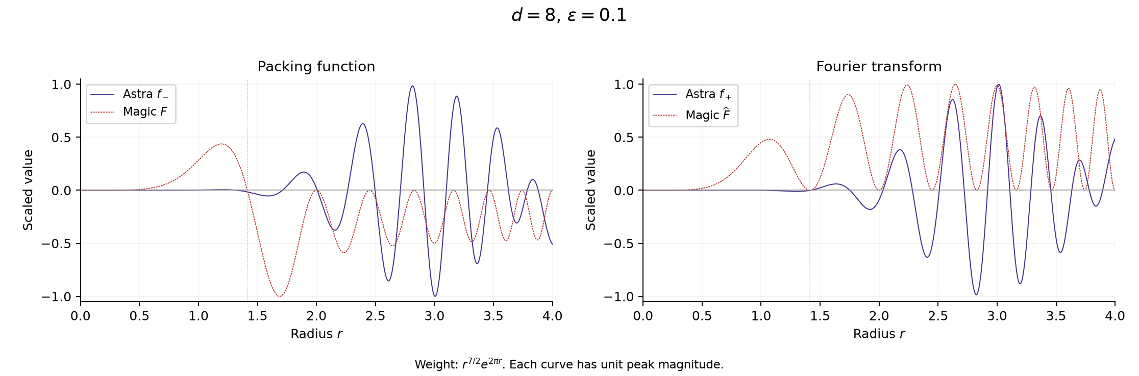
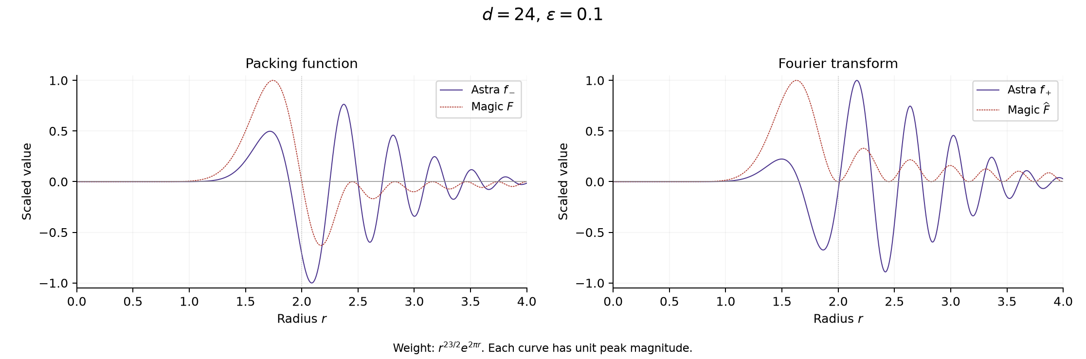
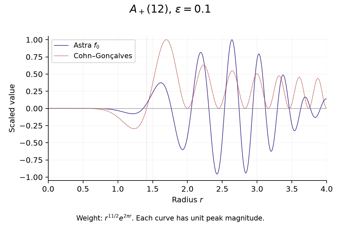
(Updated: 2026.09.20) The following plots compare the magic functions in dimensions $d = 8, 12, 24$ with the auxiliary functions $f_-$, $f_+$, and $f_0$ for $\epsilon = 0.1$. Each curve is scaled by $r^{(d-1)/2}\exp(2\pi r)$ and then peak-normalized. They show that the auxiliary functions change sign repeatedly and fail to satisfy the required nonpositivity or nonnegativity conditions. The plots don’t change much if we take a smaller $\epsilon$. The construction guarantees the desired sign conditions only for sufficiently large $d$ and does not give optimal constants in low dimensions.

Proofs of lemmas

Lemma 4.2

Lemma 4.2. There are absolute constants $\epsilon_0, c, C > 0$ such that, for every $0 < \epsilon < \epsilon_0$ and for all $\lambda > 0$, $-1 < u \le U$, and $a_0 \le a \le A$, we have

\[\lambda |w_s(a)| \cosh(ua) \le (1 - c\epsilon) \mu_{\lambda,u}(a).\]

At $u = u_0$, we have

\[\begin{align*} \int_{a_0}^{A} w_s(a) a\sinh (u_0 a) \mathrm{d}a = - \frac{1}{2} \log \frac{\pi}{2} + O(\epsilon), \\ 0 \le \int_{B}^{B+1} w_B(a) a \sinh(u_0 a) \mathrm{d}a \le Ce^{-c/\epsilon^2}. \end{align*}\]

The cutoffs satisfy

\[a_0=o(\epsilon),\qquad \frac{e^{-2A}}{A}=o(\epsilon),\qquad \epsilon A=o(1),\qquad A=o(B).\]

In particular, $0<b(a)<1$ on $[a_0,A]$ and $B>A+1$ for sufficiently small $\epsilon$. To prove the decay bound, divide the negative density by the gamma density:

\[\frac{\lambda|w_s(a)|\cosh(ua)}{\mu_{\lambda,u}(a)} =b(a)\frac{1-e^{-2a/\lambda}}{2a/\lambda} e^{(u-1)a}\frac{\cosh(ua)}{\cosh a}.\]

The fraction involving $\lambda$ is at most $1$. For $-1<u\le1$, the last two factors are also at most $1$, so the ratio is at most $b(a)\le1-2\epsilon$. For $1\le u\le U$, use $\cosh(ua)\le e^{(u-1)a}\cosh a$ and $2(U-1)=\epsilon$ to bound the ratio by

\[b(a)e^{\epsilon a} \le e^{-2\epsilon(1+a)+\epsilon a} \le e^{-2\epsilon}\le1-c\epsilon.\]

For the radius estimate, the parts omitted from the ideal weight satisfy

\[\int_0^{a_0}|w_\ast(a)|a\sinh a\,\mathrm{d}a=O(a_0),\qquad \int_A^\infty|w_\ast(a)|a\sinh a\,\mathrm{d}a =O\left(\frac{e^{-2A}}{A}\right).\]

These are $o(\epsilon)$. Multiplication by $b(a)$ changes the integral by $O(\epsilon)$, and replacing $\sinh a$ by $\sinh(u_0a)$ costs another $O(\epsilon)$ because $u_0-1=\epsilon/4$. Thus the first integral in the statement differs from the ideal value $-\frac12\log(\pi/2)$ by only $O(\epsilon)$.

For the positive term, $\sinh(u_0a)/\cosh a\le e^{(u_0-1)a}$ bounds its contribution by

\[(B+1)Qe^{(u_0-1)(B+1)} =(B+1)e^{-1/(8\epsilon^2)+\epsilon/4} \le Ce^{-c/\epsilon^2}.\]

This is where choosing $q_\epsilon>u_0-1$ makes the effect of $w_B$ on the radius negligible. $\square$

Lemma 4.3

Since $w$ is integrable and compactly supported, $h_\epsilon$ is even and entire, and is bounded on every fixed horizontal strip. In the inverse Mellin transform

\[f_j(r) = \frac{r^{-\lambda}}{2\pi} \int_{\mathbb{R}} X_{f_j}(t) r^{it} \mathrm{d}t = \frac{r^{-\lambda}}{2\pi} \int_{\mathbb{R}} \pi^{\frac{it}{2}} \Gamma\left(\frac{\lambda - it}{2}\right) e^{\lambda h(t/\lambda)}P_j\left(\frac{t}{\lambda}\right) r^{it} \mathrm{d}t,\]

the only possible poles of the integrand come from the gamma function. They occur at

\[\frac{\lambda - it}{2} = -n \Leftrightarrow t = -i(\lambda + 2n), \quad n \in \mathbb{Z}_{\ge 0}.\]

In particular, their imaginary parts are at most $-\lambda<0$. Using the asymptotic formula for the gamma function, we have

\[|X_{f_j}(s + i\tau)| \le C (1 + |s|)^{(\lambda + \tau - 1)/2 + 3} e^{-\pi|s|/4}\]

for $C=C_{d,\tau,h}>0$, so the integrand decays as $|s|\to\infty$. The same estimate holds uniformly as $\tau$ varies over a compact pole-free interval, so the integrals over the vertical sides of a rectangular contour tend to zero. We can therefore shift the contour from $\mathbb{R}$ to $\mathbb{R}+i\tau$ for any $\tau>0$, giving

\[f_j(r) = \frac{r^{-\lambda}}{2\pi} \int_{\mathbb{R}} X_{f_j}(s + i\tau) r^{i(s + i\tau)} \mathrm{d}s = \frac{r^{-\lambda -\tau}}{2\pi} \int_{\mathbb{R}} X_{f_j}(s + i\tau) r^{is} \mathrm{d}s.\]

Hence $\lvert f_j(r)\rvert=O_\tau(r^{-\lambda-\tau})$ for any $\tau>0$ as $r\to\infty$, which shows that $f_j$ is rapidly decreasing. The same argument applies to its derivatives.

For the values at the origin, we shift the contour downward to $\mathbb{R}-i(\lambda+1)$ (any height strictly between $-\lambda-2$ and $-\lambda$ would work). Then we pick up the residue at $t = -i\lambda$, which is

\[\mathrm{Res}_{t = -i\lambda} X_{f_j}(t) r^{it} = \pi^{\frac{\lambda}{2}} e^{\lambda h(-i)} P_j(-i)r^{\lambda} \cdot \mathrm{Res}_{t=-i\lambda} \Gamma\left(\frac{\lambda - it}{2}\right) = 2i\pi^{\frac{\lambda}{2}} e^{\lambda h(-i)} P_j(-i) r^{\lambda}.\]

Hence we have

\[\begin{align*} f_j(r) &= \frac{r^{-\lambda}}{2\pi} \left(-2\pi i \cdot 2i\pi^{\frac{\lambda}{2}} e^{\lambda h(-i)} P_j(-i) r^{\lambda} + r^{\lambda + 1}\int_{\mathbb{R}} X_{f_j}(s - i(\lambda + 1)) r^{is} \mathrm{d}s\right) \\ &= 2 \pi^{\frac{\lambda}{2}} e^{\lambda h(-i)} P_j(-i) + \frac{r}{2\pi} \int_{\mathbb{R}} X_{f_j}(s - i(\lambda + 1)) r^{is} \mathrm{d}s. \end{align*}\]

The second term vanishes as $r\to0$, so

\[f_j(0) = 2 \pi^{\frac{\lambda}{2}} e^{\lambda h(-i)} P_j(-i).\]

In particular, $f_+(0)=f_-(0)=2\pi^{\lambda/2}e^{\lambda h(-i)}\beta>0$, while $f_0(0)=0$. Shifting farther down gives expansions in even powers $r^{2n}$, with remainders of arbitrarily high order, including after differentiation. This proves smoothness at the origin as a radial function on $\mathbb{R}^d$. Finally, the evenness of $h$ and the reflection identities for $P_j$ give the Fourier symmetries, while conjugate symmetry of the Mellin data makes the functions real-valued. $\square$

Lemmas 4.4–4.7

These four lemmas are used in Lemma 4.8 to show that $f_j(r)$ has the same sign as $P_j(iu)$ for sufficiently large $d$ over the relevant range of $u$. The proofs are elementary but technical, so I’ll state the results and briefly indicate how the parameters enter the estimates.

Let $\delta=u-1$ and $\eta=1+u$. The lemmas use the following quantities (with our notation for $\mu_{\lambda,u}$):

\[\begin{align*} V_\gamma&=\frac1\lambda\int_0^\infty a^2\mu_{\lambda,u}(a)\,\mathrm{d}a =\frac\lambda4\psi^{(1)}\left(\frac{\lambda\eta}{2}\right),\\ M_3&=\frac1\lambda\int_0^\infty a^3\mu_{\lambda,u}(a)\,\mathrm{d}a +\int_0^\infty (|w_s(a)|+w_B(a))a^3\cosh(ua)\,\mathrm{d}a,\\ D_s(T)&=\lambda\int_{a_0}^A |w_s(a)|\cosh(ua)(1-\cos(aT))\,\mathrm{d}a,\\ D_B(T)&=\lambda\int_B^{B+1}w_B(a)\cosh(ua)(1-\cos(aT))\,\mathrm{d}a,\\ V_s&=\int_{a_0}^A|w_s(a)|a^2\cosh(ua)\,\mathrm{d}a,\qquad V_B=\int_B^{B+1}w_B(a)a^2\cosh(ua)\,\mathrm{d}a. \end{align*}\]

Thus $D_u=D_\gamma-D_s+D_B$ and $V(u)=V_\gamma-V_s+V_B$. The quantity $M_3$ bounds the cubic error without relying on cancellation between the positive and negative terms.

Lemma 4.4. There are absolute constants $c, C > 0$ such that, for every $\lambda > 0$, $u > -1$ satisfying $\lambda(1 + u) \ge 1$, and $T \in \mathbb{R}$, we have

\[\left\lvert \mathcal{L}_u(T) + \frac{\lambda V(u)}{2} T^2 \right\rvert \le C \lambda M_3 |T|^3\]

Moreover,

\[\begin{align*} \frac{1}{2\eta} &\le V_\gamma \le \frac{C}{\eta}, \\ \frac{1}{\lambda} \int_0^{\infty} a^3 \mu_{\lambda,u}(a) \mathrm{d} a &\le \frac{C}{\eta^2}, \\ D_\gamma(T) &\ge c\lambda \min \left\lbrace \frac{T^2}{\eta}, |T| \right\rbrace, \qquad (T \in \mathbb{R}). \end{align*}\]

Lemma 4.5. There is $\epsilon_0>0$ and an absolute $c>0$ such that, for every $0<\epsilon<\epsilon_0$, there are constants $C_\epsilon,\lambda_\epsilon>0$ with the following property. For every $\lambda\ge\lambda_\epsilon$ and $u_\ast\le u\le U$,

\[\begin{align*} \lambda |w_s(a)| \cosh(ua) &\le (1 - c\epsilon) \mu_{\lambda,u}(a), \qquad &(a_0 \le a \le A) \\ D_u(T) &\ge c\epsilon D_\gamma(T), \qquad &(T \in \mathbb{R}) \\ \frac{c\epsilon}{\eta} &\le V(u) \le \frac{C_\epsilon}{\eta}, \\ M_3 &\le \frac{C_\epsilon}{\eta^2}. \end{align*}\]

Moreover, $\lambda\eta\ge(\log\lambda)/4$.

The choice $U=1+\epsilon/2$ keeps the negative term below the gamma contribution throughout this range, by Lemma 4.2. For $u\ge U$, we instead use the positive term to control the negative one. Write

\[C_0=A+a_0^{-1},\qquad \rho_\epsilon=C_0Q^{-1}e^{-(U-1)(B-A)}.\]

With the chosen parameters,

\[\rho_\epsilon=C_0e^{-1/(8\epsilon^2)+(\epsilon/2)A} \le Ce^{-c/\epsilon^2}.\]

This is where $q_\epsilon<U-1$ and the separation $A=o(B)$ are used: they make the negative contribution small relative to the positive one in the following lemma.

Lemma 4.6. There are absolute constants $c, C > 0$ and $\epsilon_0 > 0$ such that, for every $0 < \epsilon < \epsilon_0$, there are constants $\lambda_\epsilon, C_\epsilon, c_\epsilon > 0$ with the following property. For every $\lambda \ge \lambda_\epsilon$ and $u \ge U$, and every $T \in \mathbb{R}$, one has

\[\begin{align*} D_s(T) &\le C \lambda C_0 e^{\delta A} \min \{T^2, 1\}, \\ D_B(T) &\ge c\lambda Q e^{\delta B} \min \{T^2, 1\}. \end{align*}\]

Consequently,

\[\begin{align*} D_s(T) &\le C \rho_\epsilon D_B(T), \\ D_u(T) &\ge D_\gamma(T) + cD_B(T), \\ cV_B &\le V(u) \le CV_B. \end{align*}\]

The positive contribution $V_B$ and the third moments satisfy

\[\begin{align*} c B^2 Q e^{\delta B} &\le V_B \le (B+1)^2 Q e^{\delta(B+1)}, \\ \int_{a_0}^{A} |w_s(a)| a^3 \cosh(ua) \mathrm{d}a &\le CA\rho_\epsilon V_B, \\ \int_{B}^{B+1} w_B(a) a^3 \cosh(ua) \mathrm{d}a &\le (B+1) V_B. \end{align*}\]

In particular,

\[M_3 \le C_\epsilon V(u), \qquad V(u) \ge c_\epsilon > 0 \quad (u \ge U).\]

Indeed, dividing the first two estimates gives, for $T\ne0$,

\[\frac{D_s(T)}{D_B(T)} \le C C_0Q^{-1}e^{-(u-1)(B-A)} \le C\rho_\epsilon.\]

Thus $U$ is where the proof switches between two sufficient decay estimates; it need not be a point where the contributions are equal.

Set $T_0=1/[2(B+1)]$.

Lemma 4.7. (Estimates for $D_u(T)$.) There is $\epsilon_0>0$ and an absolute $c>0$ such that, for every $0<\epsilon<\epsilon_0$, there are constants $c_\epsilon,\lambda_\epsilon>0$ with the following property. For every $\lambda\ge\lambda_\epsilon$ and $u\ge U$, set $\eta=1+u$ and $\delta=u-1$. Then

\[\begin{align*} D_u(T) &\ge c_\epsilon \lambda V(u) T^2, \qquad &(|T| \le T_0) \\ D_u(T) &\ge c_\epsilon \lambda Q e^{\delta B}, \qquad &(T_0 \le |T| \le \eta) \\ D_u(T) &\ge c \lambda |T| + c_\epsilon \lambda Q e^{\delta B}, \qquad &(|T| \ge \eta). \end{align*}\]

Lemma 4.8

We divide the integral into two parts, with small and large $\lvert T\rvert$, and show that the first dominates the second. More precisely, we choose

\[T_* = \frac{K}{\sqrt{\lambda V(u)}}.\]

Here $K$ may depend on $d$ and $u$, and will tend to infinity uniformly over the relevant range of $u$ as $d\to\infty$. By Lemma 4.4, we have

\[\mathcal{L}_u(T) = -\frac{\lambda V(u)}{2} T^2 + O(\lambda M_3 |T|^3)\]

and the approximation becomes uniform if the interval shrinks and the cubic error term tends to zero:

\[T_* = o_\epsilon(1), \qquad \frac{K^3 M_3}{\sqrt{\lambda} V(u)^{3/2}} = o_\epsilon(1).\]

On the ranges of $u$ stated in Lemma 4.8, the polynomials $P\in\lbrace P_-,P_+,P_0\rbrace$ have fixed degrees and satisfy

\[\frac{|P(T + iu)|}{|P(iu)|} \ll_\epsilon 1 + |T|^3, \qquad \frac{P(T + iu)}{P(iu)} = 1 + O_\epsilon(|T| + |T|^3)\]

uniformly in $u$. Thus the integral over $[-T_\ast,T_\ast]$ can be approximated by

\[\begin{align*} \int_{|T| \le T_*} e^{\mathcal{L}_u(T)} P(T + iu) \mathrm{d}T &= \int_{|x| \le K} e^{\mathcal{L}_u(x/\sqrt{\lambda V(u)})} P\left(\frac{x}{\sqrt{\lambda V(u)}} + iu\right) \frac{\mathrm{d}x}{\sqrt{\lambda V(u)}} \\ &\approx \int_{|x| \le K} e^{-\frac{\lambda V(u)}{2} \frac{x^2}{\lambda V(u)}} P(iu) \frac{\mathrm{d}x}{\sqrt{\lambda V(u)}} \\ &= P(iu) \sqrt{\frac{2\pi}{\lambda V(u)}} (1 + o_\epsilon(1)). \end{align*}\]

To make the approximation precise, the two uniform error bounds above give $e^{\mathcal{L}_u(x/\sqrt{\lambda V(u)})}=e^{-x^2/2}(1+o_\epsilon(1))$ and $P(x/\sqrt{\lambda V(u)}+iu)=P(iu)(1+o_\epsilon(1))$ for $|x|\le K$. We can pull these uniform relative errors outside the integral, and $\int_{-K}^K e^{-x^2/2}\,\mathrm{d}x\to\sqrt{2\pi}$ because $K\to\infty$.

It remains to show that the integral over $\lvert T\rvert > T_*$ becomes negligible as $d \to \infty$, i.e., that it is $o_\epsilon(\lvert P(iu) \rvert / \sqrt{\lambda V(u)})$. Here are the choices of $K$ that make both the approximation and the tail bounds work.

For $u_\ast\le u\le U$, put $L=\lambda(1+u)\ge(\log\lambda)/4$ and take $K=L^{1/12}$. Lemma 4.5 gives $V(u)\asymp_\epsilon(1+u)^{-1}$ and $M_3\ll_\epsilon(1+u)^{-2}$, so

\[\frac{T_\ast}{1+u}\ll_\epsilon L^{-5/12},\qquad \frac{K^3M_3}{\sqrt\lambda V(u)^{3/2}}\ll_\epsilon L^{-1/4}.\]

Both tend to zero uniformly. Between $T_\ast$ and $1+u$, the quadratic decay from Lemmas 4.4–4.5 gives a normalized tail of size $O_\epsilon(e^{-c_\epsilon K^2})$; beyond $1+u$, the linear decay gives $O_\epsilon(e^{-c_\epsilon L})$. These are ordinary Gaussian and exponential tail estimates. For instance,

\[\int_K^\infty e^{-cx^2}\,\mathrm{d}x \le \frac1K\int_K^\infty xe^{-cx^2}\,\mathrm{d}x =\frac{e^{-cK^2}}{2cK}\qquad(K>0).\]

For $u\ge U$, take $K=\lambda^{1/12}$. Lemma 4.6 gives $V(u)\ge c_\epsilon>0$ and $M_3\ll_\epsilon V(u)$, so $T_\ast\ll_\epsilon\lambda^{-5/12}$ and the cubic error is $O_\epsilon(\lambda^{-1/4})$. The quadratic bound in Lemma 4.7 handles $T_\ast<|T|\le T_0$. Beyond $T_0$, the factor $e^{-c_\epsilon\lambda Qe^{(u-1)B}}$ makes the integral small even as $u\to\infty$; its decay absorbs the growth of $\sqrt{V(u)}$ and the polynomial factors. For $|T|\ge1+u$, the additional exponential decay in $|T|$ makes the remaining tail integrable. Thus the tails are negligible uniformly in both ranges. $\square$

To obtain the signs of $f_j$, recall that

\[P_+(iu)=\beta+(1-u)^2(1+u),\qquad P_-(iu)=\beta-(u-1)(1+u)^2,\qquad P_0(iu)=u^2-1.\]

The first is positive for every $u>-1$. Our choice $\beta=u_0-1>0$ gives

\[P_-(iu_0)=-\beta(3+4\beta+\beta^2)<0,\qquad P_0(iu_0)=\beta(2+\beta)>0,\]

and these signs persist for all $u\ge u_0$. For sufficiently large $d$, Lemma 4.8 and the positive prefactor in the inverse Mellin formula transfer these signs to $f_j(e^{v(u)})$. Since $v^{\prime}(u)=V(u)>0$ and $v(u)\to\infty$, this gives $f_+(r)>0$ for $r\ge r_\ast$, and $f_-(r)<0<f_0(r)$ for $r\ge R_{\epsilon,d}=e^{v(u_0)}$. Thus $u_0$ is a cutoff from which the exterior signs are guaranteed, not an exact sign-change point.

Lemma 4.10

We want to show that $f_+(r)$ is close to the scaled Gaussian $f_+(0)e^{-y}$, where $y=\pi r^2e^{2h_1^{\prime}}$, and hence is positive for $0\le r\le r_\ast$. The idea is the following: we shift the contour of integration downward from $\mathbb{R}$ to $\mathbb{R} - i(\lambda + 2p)$ for $p = N + 1/2$, where $N$ is a large (but not too large) integer. Then we can write $f_+(r) / f_+(0)$ as a sum of residues at the poles in the strip, plus an integral over the shifted contour. The sum will approximate the Taylor expansion of $e^{-y}$, and the integral will be small enough to be negligible.

There are $N+1$ poles in the strip, at $t = -i(\lambda + 2n)$ for $n = 0, 1, \ldots, N$, and we pick up their residues. By applying the residue theorem to $f_+(r) / f_+(0)$, we have

\[\begin{align*} \frac{f_+(r)}{f_+(0)} &= \frac{r^{-\lambda}}{2\pi f_+(0)} \int_{\mathbb{R}} X_{f_+}(t) r^{it} \mathrm{d}t \\ &= \frac{r^{-\lambda}}{2\pi f_+(0)} \left[-2\pi i \sum_{n=0}^{N} \mathrm{Res}_{t = -i(\lambda + 2n)} (X_{f_+}(t) r^{it}) + \int_{\mathbb{R} - i(\lambda + 2N + 1)} X_{f_+}(t) r^{it} \mathrm{d}t\right] \\ &= \sum_{n=0}^{N} \frac{(-y)^n}{n!} A_{\lambda, n} + \mathcal{R}_{\lambda}(r). \end{align*}\]

The residues can be computed as follows:

\[\begin{align*} &\mathrm{Res}_{t = -i(\lambda + 2n)} (X_{f_+}(t) r^{it}) \\ &= \pi^{\frac{\lambda}{2} +n} e^{\lambda h(-i(1 + 2n/\lambda))} P_+(-i(1 + 2n/\lambda)) r^{\lambda + 2n} \cdot \mathrm{Res}_{t=-i(\lambda + 2n)} \Gamma\left(\frac{\lambda - it}{2}\right) \\ &= 2i \cdot \frac{(-1)^n}{n!} \pi^{\frac{\lambda}{2} + n} e^{\lambda h(-i(1 + 2n/\lambda))} P_+(-i(1 + 2n/\lambda)) r^{\lambda + 2n}. \end{align*}\]

Thus the coefficients and remainder in the residue expansion are

\[\begin{align*} A_{\lambda, n} &= \exp\left(\lambda [h(i(1 + 2n/\lambda)) - h(i)] - 2n h_1'\right) \frac{P_+(-i(1 + 2n/\lambda))}{P_+(-i)}, \\ \mathcal{R}_{\lambda}(r) &= \frac{\pi^{\frac{\lambda}{2} + p}r^{2p}}{2\pi f_+(0)} \int_{\mathbb{R}} \pi^{\frac{is}{2}} \Gamma\left(-p - \frac{is}{2}\right) e^{\lambda h(s/\lambda - i(1 + 2p/\lambda))} P_+\left(\frac{s}{\lambda} - i\left(1+\frac{2p}{\lambda}\right)\right) r^{is} \mathrm{d}s. \end{align*}\]

We want $N$ to be small enough that $N^2/\lambda=o(1)$. Taylor expansion of $h$ and $P_+$ then gives, uniformly for $0\le n\le N$,

\[\lambda \left[ h\left(i\left(1 + \frac{2n}{\lambda}\right)\right) - h(i)\right] = 2nh_1' + O_\epsilon\left(\frac{n^2}{\lambda}\right), \qquad \frac{P_+(-i(1 + 2n/\lambda))}{P_+(-i)} = 1 + O_\epsilon\left(\frac{n}{\lambda}\right).\]

It follows that

\[|A_{\lambda, n} - 1| = O_{\epsilon} \left(\frac{n(1+n)}{\lambda}\right)\]

for $0\le n\le N$, so the sum is close to the degree-$N$ Taylor polynomial of $e^{-y}$.

The remainder $\mathcal{R}_\lambda(r)$ is bounded using the reflection formula for the gamma function and the definition of $h$. Together with the omitted terms of the exponential series, this gives three error estimates:

\[\begin{align*} e^y \sum_{n=1}^{N} \frac{y^n}{n!} |A_{\lambda, n} - 1| &\ll_\epsilon \frac{(1+y)^2 e^{2y}}{\lambda}, \\ e^y |\mathcal{R}_{\lambda}(r)| &\ll_\epsilon \frac{e^y y^p}{\Gamma(1+p)}, \\ e^y \sum_{n > N} \frac{y^n}{n!} &\ll_\epsilon \frac{e^y y^{N+1}}{(N+1)!}. \end{align*}\]

The choice of $u_\ast$, together with the digamma asymptotic, gives

\[y \le y(r_\ast) = \frac{1}{8} \log \lambda + O_\epsilon(1).\]

Taking $N=\lceil\log\lambda\rceil$ satisfies $N^2/\lambda=o(1)$ and makes all three displayed relative errors tend to zero uniformly throughout this growing interval. The exponential-series tail estimate uses $y/(N+2)\le1/2$, which holds uniformly for these choices. In particular, Stirling’s formula bounds the logarithm of either tail by $(1/8+1-\log8)\log\lambda+O_\epsilon(\log\log\lambda)$, whose leading coefficient is negative. Thus

\[\frac{f_+(r)}{f_+(0)} = e^{-y} \left(1 + O_\epsilon\left(\frac{(\log \lambda)^2}{\lambda^{3/4}}\right)\right)\]

uniformly on $0 \le r \le r_\ast$. $\square$

Appendix

(Updated 2026.09.21) There is an interesting result in the appendix of the report, which is not used in the proof of the main theorem.

Proposition A.1. For $d \ge 1$, we have $\mathsf{A}_+(d) < \mathsf{A}_-(d)$.

The proof is quite interesting: the main idea is to considering the integral operator

\[(T_d g)(x) = \frac{\lambda}{2} \int_1^\infty t^{\lambda - 1} g(tx) \mathrm{d}t.\]

The proof shows that, if $g \in L^{1}_{\mathrm{rad}}(\mathbb{R}^d; \mathbb{R})$ satisfies $g(0) = 0$ and $\widehat{g} = -g$, then $T_d g$ (with $(T_d g)(0) := 0$) becomes a self-Fourier function, i.e. $\widehat{T_d g} = T_d g$. (I think the normalization factor $\lambda / 2$ is chosen so that $\lVert T_d g \rVert_1 \le \frac{1}{2} \lVert g \rVert_1$ holds.) From $\widehat{g} = -g$, the Mellin transform of $g$ vanishes at the center — $\int_0^\infty g(r) r^{\lambda - 1} \mathrm{d}r = 0$ — and this proves $\widehat{T_d g} = T_d g$. Now, the important fact is that $r(T_d g) < r(g)$, which is almost immediate from the definition of $T_d$: if $g(r) \ge 0$ for all $r \ge R = r(g)$, then

\[(T_d g)(r) = \frac{\lambda}{2} r^{-\lambda} \int_r^\infty s^{\lambda - 1} g(s) \mathrm{d}s \ge 0 \quad (r \ge R),\]

and hence $r(T_d g) \le R$. If equality holds, then $g$ must vanish on $[R, \infty)$, which is impossible since any function $f$ where both $f$ and $\widehat{f}$ are compactly supported must be identically zero. Now the claim follows from the fact that there an extremizer for $\mathsf{A}_-(d)$, i.e. $g$ with $r(g) = \mathsf{A}_-(d)$ and $\widehat{g} = -g$, which is Theorem 1.4 of Cohn-Gonçalves.

Formalization

There’s also an accompanying formalization of the proof in Lean. How faithfully does it reflect the report? See Part 2.

Use of LLMs

LLMs—mostly ChatGPT—were used to help me understand the original proof and the formalization. In particular, I had a conversation with ChatGPT in the Codex app where I mostly asked questions about the intuition and choice of parameters in the proof. For example, I asked why the perturbation $h$ is chosen to have the form $h(\zeta) = \int_0^\infty w(a) (\cos(a\zeta) - 1) \mathrm{d} a$, and why $u_\ast$ is chosen as $-1 + \frac{\log \lambda}{4\lambda}$, not something like $-1 + \frac{\log \lambda}{2\lambda}$ or $-1 + \delta$ for some fixed $\delta > 0$. Most of the proofs are very analytical, and the technical details are mostly about “how to choose the right parameters so that this is larger than that”.

Tags: math  ai