Understanding Astra's result on high-dimensional sphere packing — Part 2: Formalization
In the previous post, I explained the main ideas behind Astra’s proof of the optimal Cohn-Elkies LP exponent and the sharp sign-uncertainty constant. OpenAI released Lean formalizations accompanying all ten results in the report, including the sphere-packing result. Here I dig into the sphere-packing formalization and ask how faithfully it follows the report: what is the same, what is different, and, more importantly, what is missing? My aim is to match the informal statements and proofs with their Lean counterparts. Comments inside the displayed Lean snippets are sometimes added for explanation and are not part of the original source.
Overview of the formalization
The Lean code can be found in SpherePacking.lean. I checked commit 94bc0fe, in which it is a single file of 55,616 lines.
- The repository includes Comparator configurations and an informative
formalization.yaml. The latter identifiesPackingBounds.sharpFullCohnElkiesManuscriptConclusionsas the main sphere-packing result and records its axiom andsorrystatus. - There are many definitions, which makes the file difficult to navigate linearly.
- On the first day of the announcement, I remember the repository being repeatedly force-pushed, so earlier versions may not be recoverable from its public Git history.
- Some parts of the code are borrowed from the sphere packing project.
- There is no blueprint explaining the dependency structure.
So how can I read 55K lines of Lean code? There are several choices:
- Do not read it.
- Spend months reading it manually and put other important work aside.
- Use AI.
I chose option 3 and used ChatGPT and Claude, relying somewhat more on ChatGPT for reading the code because the Lean code was itself produced by an OpenAI model. I asked the models to build a table matching the theorems and lemmas in the report with declarations in the Lean file, and then checked the suggested declarations against the source.
In short, the file proves the result on the exponent of the Cohn-Elkies LP bound (Theorem 1.1). However, several intermediate results and half of Theorem 1.2 are missing. More precisely:
- Section 2.1 of the report discusses radial and $L^1$-to-Schwartz reductions. The formalization prove radial reduction for the Schwartz LP problem, but it does not prove the $L^1$-to-Schwartz reduction.
- The definition of $\mathsf{A}_+(d)$ is missing. The formalization considers anti-self-Fourier functions and Fourier pairs, but not self-Fourier functions. In particular, it only formalizes half of Theorem 1.2.
- Proposition A.1 of the appendix is not formalized (which is obvious, considering that $\mathsf{A}_+(d)$ is not formalized).
The absence of these results makes sense if you imagine that Astra’s main goal is to prove the optimal Cohn-Elkies exponent. The sign uncertainty principle naturally arises in this argument, but $\mathsf{A}_+(d)$ is not needed.
Also, some of the proofs are slightly modified.
- The original proof of Lemma 3.2 (bounding the normalized Mellin transform) uses the Poisson inequality for upper half plane for subharmonic functions, while the formalization uses Phragmén-Lindelöf principle on a strip instead.
- In the formalization of the proof of upper bound, the parameters used in the construction of auxiliary function $w(a)$ ($a_0, A, b(a)$) are chosen differently from the report.
Now, let’s read the Lean code!
Basic definitions
Some basic definitions, including the Schwartz space and radiality, are formalized as follows:
abbrev Euclidean (d : ℕ) := EuclideanSpace ℝ (Fin d)

abbrev TestFunction (d : ℕ) := 𝓢(Euclidean d, ℂ)

def IsRealValued {d : ℕ} (f : TestFunction d) : Prop :=
  ∀ x : Euclidean d, (f x).im = 0

def IsRadial {d : ℕ} (f : TestFunction d) : Prop :=
  ∀ x y : Euclidean d, ‖x‖ = ‖y‖ → f x = f y

structure AntiFourierWitness (d : ℕ) (R : ℝ) where
  function : TestFunction d
  real : IsRealValued function
  radial : IsRadial function
  nonzero : function ≠ 0
  anti_fourier : (𝓕 function : TestFunction d) = -function
  zero_value : function (0 : Euclidean d) = 0
  eventually_nonneg :
    ∀ x : Euclidean d, R ≤ ‖x‖ → 0 ≤ (function x).re
An AntiFourierWitness is the main object in the formal lower-bound argument. It consists of a nonzero real-valued radial Schwartz function $g$ satisfying $\widehat g=-g$, $g(0)=0$, and $g(x)\ge0$ for $\lVert x\rVert\ge R$. There is no analogous “SelfFourierWitness” for $\widehat g=g$ in the Lean file.
Lower bound
The main goal of the lower-bound argument is to prove the following statement:
def criticalRadius : ℝ := (Real.pi)⁻¹

def UniformAntiFourierSignRadius : Prop :=
  ∀ c : ℝ, 0 < c → c < criticalRadius →
    ∀ᶠ d : ℕ in atTop,
      IsEmpty (AntiFourierWitness d (c * Real.sqrt (d : ℝ)))
Note that it has a dedicated name for the constant $1/\pi$, criticalRadius!
UniformAntiFourierSignRadius asserts that for every $0<c<1/\pi$, there exists a dimension threshold $d_0(c)$ such that, for all $d\ge d_0(c)$, there is no nonzero radial Schwartz function $g$ satisfying $\widehat g=-g$, $g(0)=0$, and $g(x)\ge0$ for $\lvert x\rvert\ge c\sqrt d$.
The final theorem supplies a proof of this proposition:
theorem uniformAntiFourierSignRadius :
    UniformAntiFourierSignRadius := by ...
To prove this, recall that we worked with the normalization $\varphi$ of $g$ and its (normalized) Mellin transform $Z$. These definitions are formalized as follows:
-- theta
def stripAngle (σ : ℝ) : ℝ :=
  Real.pi * (1 + σ) / 2

-- P_σ
def stripPoissonKernel (σ T : ℝ) : ℝ :=
  Real.sin (stripAngle σ) /
    (4 * (Real.cosh (Real.pi * T / 2) - Real.cos (stripAngle σ)))

-- M_σ
def stripBottomMass (σ : ℝ) : ℝ :=
  (1 - σ) / 2

-- |S_d|
def radialSurfaceArea (d : ℕ) : ℝ :=
  (d : ℝ) * unitBallVolume d

-- ||g||_1
def radialL1Mass {d : ℕ} (g : TestFunction d) : ℝ :=
  ∫ x : Euclidean d, ‖g x‖

def radialUnitDirection {d : ℕ} (hd : 0 < d) : Euclidean d :=
  (EuclideanSpace.basisFun (Fin d) ℝ) ⟨0, hd⟩

def radialProfile {d : ℕ} (hd : 0 < d)
    (f : TestFunction d) (r : ℝ) : ℂ :=
  f (r • radialUnitDirection hd)

-- M
def radialMellinStrip {d : ℕ}
    (hd : 0 < d) (f : TestFunction d) (z : ℂ) : ℂ :=
  mellin (radialProfile hd f)
    ((d : ℂ) / 2 - Complex.I * z)

-- Z
def normalizedRadialMellinStrip {d : ℕ}
    (hd : 0 < d) (f : TestFunction d) (R : ℝ) (z : ℂ) : ℂ :=
  (radialSurfaceArea d / radialL1Mass f : ℝ) *
    Complex.exp
      (((d : ℂ) / 2 + Complex.I * z) *
        (Real.log R : ℂ)) *
      radialMellinStrip hd f z

-- φ
def normalizedRadialLogProfile {d : ℕ} (hd : 0 < d)
    (g : TestFunction d) (R v : ℝ) : ℝ :=
  radialSurfaceArea d / radialL1Mass g *
    (R * Real.exp v) ^ d *
    (radialProfile hd g (R * Real.exp v)).re
The paper’s main analytic estimate for the lower bound is Proposition 3.1:
Proposition 3.1. For every $0<c<1/\pi$, there exist $C_c,\gamma_c>0$ and $d_0(c)\in\mathbb N$ such that, for every $d\ge d_0(c)$, every $\varsigma\in\lbrace-1,+1\rbrace$, and every nonzero $g\in\mathcal S_{\mathrm{rad}}(\mathbb R^d;\mathbb R)$ satisfying $\widehat g=\varsigma g$ and $g(0)=0$, one has
\[\int_{|x| < c \sqrt{d}} |g(x)| \mathrm{d}x \le C_c e^{-\gamma_c d} \|g\|_1.\]
There is no theorem stating Proposition 3.1 in this form.
Instead, it is stated in terms of $\varphi$ (see below).
Lean proves the estimates needed for an AntiFourierWitness: besides $\widehat g=-g$, this already assumes $g(x)\ge0$ outside the given radius. This is sufficient for the LP lower bound, but it is not equivalent to Proposition 3.1, even after restricting that proposition to $\varsigma=-1$.
Here is a summary of the actual formal argument.
Proof (Lean). One checks that $\lVert \varphi\rVert_1=1$, $\int\varphi=0$, and $\varphi(v)\ge0$ for $v\ge0$. Therefore
\[\int_{-\infty}^{0} |\varphi(v)| \mathrm{d}v \ge \frac{1}{2}.\]There exists $D_0\in\mathbb R$ such that, for every $D\ge D_0$, every $-1<\sigma<1$, and every $s\in\mathbb R$, the normalized Mellin transform satisfies
\[|Z(s + i\sigma\lambda)| \le e^{H_{\sigma, D}(s)}\]where
\[H_{\sigma,D}(s)=\int_{\mathbb R}P_\sigma(T)\min\{h_\lambda(s-\lambda T),D\}\,\mathrm dT\le H_\sigma(s).\]We can show that $H_\sigma(s)$ is maximized at $s=0$. For $0\le\sigma<1$, the formalized bound for $H_\sigma(0)$ is
\[\begin{align*} H_\sigma(0) &\le \lambda M_\sigma \underbrace{\left(\log(2\pi e c^2) + \int_{\mathbb{R}} \frac{P_\sigma(T)}{M_\sigma} \left(-\frac{\pi|T|}{4} - \frac{1}{2} \log \left(1 + \frac{T^2}{4}\right) + \frac{|T|}{2} \arctan \left(\frac{|T|}{2}\right)\right)\mathrm{d}T\right)}_{A_\sigma} \\ &\quad + \int_{\mathbb{R}} P_\sigma(T) \left(3 \left|\log \frac{|T|}{2}\right| + \log\left(1 + \frac{T^2}{4} \right) + \frac12 \log\coth\frac{\pi|T|}{2}\right) \mathrm{d}T \end{align*}\]Taking $\sigma \to 1^{-}$ on the right-hand side gives
\[\lim_{\sigma \to 1^{-}} \frac{P_\sigma(T)}{M_\sigma} = \frac{\pi}{4\left(\cosh\frac{\pi T}{2} + 1\right)}, \qquad \lim_{\sigma \to 1^{-}} A_\sigma = \log(\pi^2 c^2)\]where the latter limit is negative when $c<1/\pi$. Hence, for any given $0<c<1/\pi$, we can choose $\sigma=\sigma(c)<1$ and $\gamma=\gamma(c)>0$ such that
\[H_\sigma(s) \le -\gamma \lambda\]for sufficiently large $\lambda = d/2$ and all $s \in \mathbb{R}$. We also have a separate logarithmic tail estimate: for suitable $A,B,\kappa>0$,
\[H_\sigma(\lambda S)\le-\kappa\lambda\log\frac{|S|}{A} \qquad (|S|\ge B).\]By averaging these two estimates, we obtain
\[e^{H_\sigma(\lambda S)} \le C \frac{e^{-\gamma\lambda}}{(1 + |S|)^2}\]for some constants $C,\gamma>0$, all sufficiently large $d$, and every $S\in\mathbb R$. Combining this with the pointwise estimate $\lvert Z(s+i\sigma\lambda)\rvert\le e^{H_\sigma(s)}$ above and then making the change of variables $s=\lambda S$, we obtain
\[\int_{\mathbb R}|Z(s+i\sigma\lambda)|\,\mathrm ds \le CJ\lambda e^{-\gamma\lambda},\]where $J=\int_{\mathbb R}(1+\lvert S\rvert)^{-2}\,\mathrm dS$. Mellin inversion gives
\[\int_{-\infty}^{0} |\varphi(v)| \mathrm{d}v \le \frac{1}{2\pi (1 - \sigma) \lambda} \int_{\mathbb{R}} |Z(s + i\sigma\lambda)| \mathrm{d}s\]and hence
\[\frac12\le\int_{-\infty}^{0}|\varphi(v)|\,\mathrm dv\le K e^{-\gamma\lambda},\]which is a contradiction for sufficiently large $\lambda = d/2$.
Here is how these steps are formalized.
The lower bound $\frac12\le\int_{-\infty}^{0}\lvert \varphi(v)\rvert\,\mathrm dv$
This straightforward step follows almost directly from the definition of $\varphi$ and the properties of $g$. The formal statement is as follows:
theorem normalizedProfile_negativeHalfline_mass_ge_half {φ : ℝ → ℝ}
    (hφ : Integrable φ)
    (hmean : (∫ v : ℝ, φ v) = 0)
    (hmass : (∫ v : ℝ, |φ v|) = 1)
    (hsign : ∀ v : ℝ, 0 ≤ v → 0 ≤ φ v) :
    (1 / 2 : ℝ) ≤ ∫ v in Iic (0 : ℝ), |φ v| := by ...
The upper bound $\lvert Z(s+i\sigma\lambda)\rvert\le e^{H_{\sigma,D}(s)}$
This is a capped version of Lemma 3.2, formalized as follows:
-- |Z(s + iσλ)| ≤ exp(∫ P_σ(T) h_{λ,D}(s - λT) dT) for sufficiently large D
theorem exists_antiFourierWitness_capped_poisson_majorization
    {d : ℕ} (hd : 0 < d) {R : ℝ} (hR : 0 < R)
    (w : AntiFourierWitness d R) :
    ∃ D₀ : ℝ,
      ∀ D : ℝ, D₀ ≤ D →
        ∀ {σ : ℝ}, -1 < σ → σ < 1 →
          ∀ s : ℝ,
            ‖normalizedRadialMellinStrip hd w.function R
              ((s : ℂ) + Complex.I *
                (((σ * ((d : ℝ) / 2) : ℝ) : ℂ)))‖ ≤
              Real.exp
                (∫ T : ℝ,
                  stripPoissonKernel σ T *
                    lowerGammaBoundaryCapped
                      ((d : ℝ) / 2) R D
                      (s - ((d : ℝ) / 2) * T)) := by ...
The truncation argument is explained in the final part of the proof of Lemma 3.2. The exponent on the right-hand side is the capped Poisson majorant
\[\int_{\mathbb{R}} P_\sigma(T) \min\{h_\lambda(s - \lambda T), D\} \mathrm{d}T\]Taking $D\to\infty$ gives the uncapped bound from Lemma 3.2. This is formalized as follows: lowerStripCappedPoisson_tendsto_radius proves convergence of the capped Poisson integrals, and antiFourierWitness_norm_le_poisson_of_eventually_capped_radius transfers the norm bound to the limit.
theorem lowerStripCappedPoisson_tendsto_radius
    {d : ℕ} (hd : 0 < d) {R σ : ℝ}
    (hσbelow : -1 < σ) (hσabove : σ < 1) (s : ℝ) :
    Tendsto
      (fun n : ℕ =>
        ∫ T : ℝ,
          stripPoissonKernel σ T *
            lowerGammaBoundaryCapped ((d : ℝ) / 2)
              R (n : ℝ)
              (s - ((d : ℝ) / 2) * T))
      atTop
      (𝓝 (lowerStripPoissonMajorant ((d : ℝ) / 2)
        R σ s)) := by ...

theorem antiFourierWitness_norm_le_poisson_of_eventually_capped_radius
    {d : ℕ} (hd : 0 < d) {R σ : ℝ}
    (w : AntiFourierWitness d R)
    (hσbelow : -1 < σ) (hσabove : σ < 1) (s : ℝ)
    (hcapped : ∀ᶠ n : ℕ in atTop,
      ‖normalizedRadialMellinStrip hd w.function R
        ((s : ℂ) + Complex.I *
          (((σ * ((d : ℝ) / 2) : ℝ) : ℂ)))‖ ≤
        Real.exp
          (∫ T : ℝ,
            stripPoissonKernel σ T *
              lowerGammaBoundaryCapped ((d : ℝ) / 2)
                R (n : ℝ)
                  (s - ((d : ℝ) / 2) * T))) :
      ‖normalizedRadialMellinStrip hd w.function R
        ((s : ℂ) + Complex.I *
          (((σ * ((d : ℝ) / 2) : ℝ) : ℂ)))‖ ≤
        Real.exp
          (lowerStripPoissonMajorant ((d : ℝ) / 2)
            R σ s) := by ...
The Lean argument proceeds as follows.
Proof (Lean). For $z\in\mathbb C$ and $y\in\mathbb R$, define
\[K_\lambda(z,y)=\frac{i}{4\lambda} \frac{\exp\left(\frac{\pi(z-y+i\lambda)}{2\lambda}\right)+1} {\exp\left(\frac{\pi(z-y+i\lambda)}{2\lambda}\right)-1},\]and
\[\widetilde K_\lambda(z,y)=K_\lambda(z,y)+ \begin{cases} \dfrac{i}{4\lambda},&y\ge0,\\ -\dfrac{i}{4\lambda},&y<0. \end{cases}\]Here $K_\lambda$ is a holomorphic version of the Poisson kernel, while $\widetilde K_\lambda$ is regularized so that $\widetilde K_\lambda(z,y)\to0$ as $\lvert y\rvert\to\infty$. Define
\[h_{\lambda,D}(y)= \begin{cases} \min\{h_\lambda(y),D\},&y\ne0,\\ D,&y=0, \end{cases}\]and
\[W_D(z) = \int_{\mathbb{R}} \widetilde{K}_\lambda(z, y) h_{\lambda, D}(y) \mathrm{d}y.\]At $z=s+i\sigma\lambda$ in the open strip, with $-1<\sigma<1$, the real part of $W_D$ is
\[\Re W_D(s+i\sigma\lambda) =\int_{\mathbb R}P_\sigma(T)h_{\lambda,D}(s-\lambda T)\,\mathrm dT.\]The function $\Re W_D$ has a continuous real-valued extension $H_D$ to the closed strip, with $H_D(s-i\lambda)=h_{\lambda,D}(s)$ and $H_D(s+i\lambda)=0$. Set $F_D(z)=e^{-W_D(z)}Z(z)$ in the open strip and $N_D(z)=e^{-H_D(z)}\lvert Z(z)\rvert$ on the closed strip. Then $F_D$ is holomorphic, $N_D$ is continuous, and $N_D=\lvert F_D\rvert$ in the interior. The boundary estimates for $Z$ give $N_D\le1$ on both boundary lines. The growth condition also needs checking: boundedness of $Z$ and the bound $\lvert\Re W_D(z)\rvert\le B(1+\lvert\Re z\rvert)$ give $\lvert F_D(z)\rvert\le C\exp(B\lvert\Re z\rvert)$, which is sufficient for the strip Phragmén-Lindelöf principle. It follows that $N_D\le1$ throughout the strip, and hence $\lvert Z(z)\rvert\le e^{\Re W_D(z)}$ in the interior.
Thus, the proof starts with the complex Poisson kernel and takes its real part to recover the Poisson kernel itself; this is another difference from the report.
Note that the code uses the variable ℓ, which is the same as $\lambda$.
-- K_λ(z,y) = i/(4λ) * (exp(π(z-y+iλ)/(2λ)) + 1)/(exp(π(z-y+iλ)/(2λ)) - 1)
-- ℓ = λ
def stripHolomorphicPoissonKernel (ℓ : ℝ) (z : ℂ) (y : ℝ) : ℂ :=
  (Complex.I *
      ((Complex.exp
          (((Real.pi : ℂ) *
            (z - (y : ℂ) + Complex.I * (ℓ : ℂ))) /
              (2 * (ℓ : ℂ))) + 1) /
        (Complex.exp
          (((Real.pi : ℂ) *
            (z - (y : ℂ) + Complex.I * (ℓ : ℂ))) /
              (2 * (ℓ : ℂ))) - 1)) /
    4) / (ℓ : ℂ)

-- K̃_λ(z,y) = K_λ(z,y) + (if 0 ≤ y then i/(4λ) else -i/(4λ))
def stripRegularizedHolomorphicPoissonKernel
    (ℓ : ℝ) (z : ℂ) (y : ℝ) : ℂ :=
  stripHolomorphicPoissonKernel ℓ z y +
    (if 0 ≤ y then Complex.I else -Complex.I) /
      ((4 * ℓ : ℝ) : ℂ)

-- W[b](z) = ∫ K̃_λ(z,y) b(y) dy
def stripRegularizedOuter (ℓ : ℝ) (b : ℝ → ℝ) (z : ℂ) : ℂ :=
  ∫ y : ℝ,
    stripRegularizedHolomorphicPoissonKernel ℓ z y *
      (b y : ℂ)

-- W_D(z) = W[h_{λ,D}](z) = ∫ K̃_λ(z,y) h_{λ,D}(y) dy
def lowerStripCappedGammaOuter
    (ℓ R D : ℝ) (z : ℂ) : ℂ :=
  stripRegularizedOuter ℓ
    (lowerGammaBoundaryCapped ℓ R D) z

-- Re K_λ(s + iσλ, y) = P_σ((s - y)/λ)/λ
theorem stripHolomorphicPoissonKernel_re
    {ℓ σ : ℝ} (hℓ : 0 < ℓ)
    (hbelow : -1 < σ) (habove : σ < 1) (s y : ℝ) :
    (stripHolomorphicPoissonKernel ℓ
      ((s : ℂ) + Complex.I * ((σ * ℓ : ℝ) : ℂ)) y).re =
      stripPoissonKernel σ ((s - y) / ℓ) / ℓ := by ...

-- Re W_D(s + iσλ) = ∫ P_σ(T) h_{λ,D}(s - λT) dT
theorem lowerStripCappedGammaOuter_re_dimension
    {d : ℕ} (hd : 0 < d) {σ R D : ℝ}
    (hσbelow : -1 < σ) (hσabove : σ < 1) (s : ℝ) :
    (lowerStripCappedGammaOuter ((d : ℝ) / 2) R D
      ((s : ℂ) + Complex.I *
        ((σ * ((d : ℝ) / 2) : ℝ) : ℂ))).re =
      ∫ T : ℝ, stripPoissonKernel σ T *
        lowerGammaBoundaryCapped
          ((d : ℝ) / 2) R D
          (s - ((d : ℝ) / 2) * T) := by ...
The informal proof in the report applies the Poisson inequality for upper half plane to the subharmonic function $\log\lvert Z\circ\Phi^{-1}\rvert$. The formalized proof is slightly different: it uses a horizontal-strip version of the Phragmén-Lindelöf principle, which is a maximum-principle argument for holomorphic functions on a horizontal strip, although the underlying argument is essentially the same.
Phragmén–Lindelöf principle for a horizontal strip. Let $f:\mathbb C\to\mathbb C$ be holomorphic on $\lbrace z:a<\Im z<b\rbrace$, and suppose its modulus has a continuous extension $N$ to the closed strip. Suppose that $\lvert f(z)\rvert=O(\exp(B\exp(c\lvert \Re z\rvert)))$ for some constants $B$ and $c$ with $c<\pi/(b-a)$, uniformly in the strip as $\lvert \Re z\rvert\to\infty$. If $N\le C$ on the two boundary lines for some $C>0$, then $N\le C$ throughout the strip.
This is a version of the maximum-modulus principle for a horizontal strip. The file proves it as horizontalStrip_norm_extension_majorization. The distinction between continuity of $f$ and continuity of its modulus matters here: the proof constructs the latter, not a continuous boundary extension of $F_D$ itself. Mathlib’s related theorem PhragmenLindelof.horizontal_strip assumes that $f$ is continuous on the closed strip, so it is not a direct replacement without additional boundary regularity.
theorem horizontalStrip_norm_extension_majorization
    {a b C : ℝ} (hab : a < b) (hC : 0 < C)
    (f : ℂ → ℂ) (N : ℂ → ℝ)
    (hf : DifferentiableOn ℂ f
      (Complex.im ⁻¹' Ioo a b))
    (hN : ContinuousOn N
      (Complex.im ⁻¹' Icc a b))
    (hNnonneg : ∀ w : ℂ,
      w.im ∈ Icc a b → 0 ≤ N w)
    (hinterior : ∀ w : ℂ,
      w.im ∈ Ioo a b → N w = ‖f w‖)
    (hbottom : ∀ w : ℂ, w.im = a → N w ≤ C)
    (htop : ∀ w : ℂ, w.im = b → N w ≤ C)
    (hgrowth :
      ∃ c < Real.pi / (b - a), ∃ B : ℝ,
        Asymptotics.IsBigO
          (Filter.comap (fun w : ℂ => |w.re|)
              Filter.atTop ⊓
            Filter.principal
              (Complex.im ⁻¹' Ioo a b))
          f
          (fun w : ℂ =>
            Real.exp (B * Real.exp (c * |w.re|))))
    {z : ℂ} (hza : a ≤ z.im) (hzb : z.im ≤ b) :
    N z ≤ C := by ...
$H_\sigma(s)\le H_\sigma(0)$
Here is the formalization of the inequality:
theorem lowerStripPoissonMajorant_dimension_centered_max
    {d : ℕ} (hd : 2 ≤ d) {c σ : ℝ}
    (hc : 0 < c)
    (hbelow : -1 < σ) (habove : σ < 1) (s : ℝ) :
    lowerStripPoissonMajorant ((d : ℝ) / 2)
      (c * Real.sqrt d) σ s ≤
      lowerStripPoissonMajorant ((d : ℝ) / 2)
        (c * Real.sqrt d) σ 0 := by ...
As mentioned in Part 1, the convolution of two even, nonnegative functions that are nonincreasing on $(0,\infty)$ is maximized at the origin. The Lean code includes a formalization of this fact, specialized to the Poisson kernel:
theorem even_antitone_poisson_convolution_max
    {σ : ℝ} (hbelow : -1 < σ) (habove : σ < 1)
    {f : ℝ → ℝ} {B : ℝ}
    (hf : Integrable f)
    (hfmeas : Measurable f)
    (hfnonneg : ∀ x : ℝ, 0 ≤ f x)
    (heven : ∀ x : ℝ, f (-x) = f x)
    (hanti : AntitoneOn f (Ici (0 : ℝ)))
    (hsupport : Function.support f ⊆ Icc (-B) B)
    (s : ℝ) :
    (∫ x : ℝ, stripPoissonKernel σ (s - x) * f x) ≤
      ∫ x : ℝ, stripPoissonKernel σ (0 - x) * f x := by ...
The function $h_\lambda$ itself is neither nonnegative nor compactly supported, so the lemma is not applied directly to it. Lean first uses the even, nonnegative, compactly supported function $q_{N,D}(Y)=\max\lbrace h_{\lambda,D}(\lambda Y)+N,0\rbrace$ (lowerGammaScaledCappedClipped). After applying the lemma, it subtracts $NM_\sigma$ and removes the lower and upper truncations by dominated convergence. Finally, lowerStripPoissonMajorant_scaled_convolution identifies the convolution at $s/\lambda$ with $H_\sigma(s)$.
$H_\sigma(0) \le \lambda M_\sigma (\log(2\pi c^2) + J_\sigma) + O_\sigma(1)$
Recall that Lemma 3.3 proves the upper bound for $H_\sigma(0)$, treating the even- and odd-dimensional cases separately in order to estimate the difference
\[h_\lambda(\lambda T) - \lambda\left(\log(2\pi c^2) - \int_0^1 f_T(x) \mathrm{d}x\right).\]The Lean proof uses the same even/odd Riemann-sum calculation, but only proves the upper estimate needed later, not the report’s full weighted absolute-error estimate (19). Its unified error, lowerRiemannPoissonError σ, is finite and independent of $d$ and $c$ for each fixed $0\le\sigma<1$. Thus lowerStripPoissonMajorant_dimension_central_bound gives a one-sided $O_\sigma(1)$ error; this does not assert a two-sided approximation.
-- f_T
def lowerRiemannLog (T x : ℝ) : ℝ :=
  Real.log (Real.sqrt (x ^ 2 + T ^ 2 / 4))

-- Combined error term
def lowerRiemannErrorMajorant (T : ℝ) : ℝ :=
  3 * |lowerRiemannLog T 0| +
    2 * |lowerRiemannLog T 1| +
      (1 / 2 : ℝ) *
        Real.log (lowerCoth (Real.pi * |T| / 2))

def lowerRiemannPoissonError (σ : ℝ) : ℝ :=
  ∫ T : ℝ,
    stripPoissonKernel σ T * lowerRiemannErrorMajorant T

-- P_σ(T)/M_σ
def stripNormalizedPoissonKernel (σ T : ℝ) : ℝ :=
  stripPoissonKernel σ T / stripBottomMass σ

def lowerEndpointPhase (T : ℝ) : ℝ :=
  -Real.pi * |T| / 4 - (1 / 2 : ℝ) * Real.log (1 + T ^ 2 / 4) +
    |T| / 2 * Real.arctan (|T| / 2)

def lowerPoissonEndpointExpectation (σ : ℝ) : ℝ :=
  ∫ T : ℝ,
    stripNormalizedPoissonKernel σ T * lowerEndpointPhase T

-- H_σ(0) ≤ λ M_σ (log(2πc^2)+J_σ) + error
theorem lowerStripPoissonMajorant_dimension_central_bound
    {d : ℕ} (hd : 2 ≤ d) {c σ : ℝ}
    (hc : 0 < c) (hzero : 0 ≤ σ) (habove : σ < 1) :
    lowerStripPoissonMajorant ((d : ℝ) / 2)
        (c * Real.sqrt d) σ 0 ≤
      ((d : ℝ) / 2) * stripBottomMass σ *
        (Real.log (2 * Real.pi * Real.exp 1 * c ^ 2) +
          lowerPoissonEndpointExpectation σ) +
        lowerRiemannPoissonError σ := by ...
There are some differences between the formalization and the report. For example, the main estimate reads
\[\begin{align*} H_\sigma(0) &\le \lambda M_\sigma \left(\log(2\pi e c^2) + \int_{\mathbb{R}} \frac{P_\sigma(T)}{M_\sigma} \left(-\frac{\pi|T|}{4} - \frac{1}{2} \log \left(1 + \frac{T^2}{4}\right) + \frac{|T|}{2} \arctan \left(\frac{|T|}{2}\right)\right)\mathrm{d}T\right) \\ &\quad + \int_{\mathbb{R}} P_\sigma(T) \left(3 |f_T(0)| + 2 |f_T(1)| + \frac12 \log\coth\frac{\pi|T|}{2}\right) \mathrm{d}T \end{align*}\]which looks different from the one in the report. In fact, for $T\ne0$, we have
\[-\int_{0}^{1} f_T(x)\mathrm{d}x = 1 + \left(-\frac{\pi|T|}{4} - \frac{1}{2} \log \left(1 + \frac{T^2}{4}\right) + \frac{|T|}{2} \arctan \left(\frac{|T|}{2}\right)\right)\]Therefore, we have
\[\log(2\pi e c^2) + \int_{\mathbb{R}} \frac{P_\sigma(T)}{M_\sigma} \left(-\frac{\pi|T|}{4} - \frac{1}{2} \log \left(1 + \frac{T^2}{4}\right) + \frac{|T|}{2} \arctan \left(\frac{|T|}{2}\right)\right)\mathrm{d}T = \log(2\pi c^2) + J_\sigma.\]theorem integral_lowerRiemannLog
{T : ℝ} (hT : T ≠ 0) :
-(∫ x in (0 : ℝ)..1, lowerRiemannLog T x) =
1 + lowerEndpointPhase T := by ...
The expression for $h_\lambda(\lambda T)$ in terms of a Riemann sum for $f_T$, together with an error estimate for that Riemann sum, is formalized by:
- for even $d$:
lowerGammaBoundaryLog_integer_scaledandlower_integer_leftRiemann_error; - for odd $d$:
lowerGammaBoundaryLog_halfInteger_scaled,lower_halfInteger_midpointRiemann_error, andlowerRiemannLog_halfInteger_tail_integral_le.
The error term is slightly different: it uses the unified bound lowerRiemannErrorMajorant for both even and odd dimensions:
(lowerCoth is just $\coth$, but with a fancier name!)
The even- and odd-dimensional cases are then combined in the proof of lowerGammaBoundaryLog_dimension_riemann_le (the proof begins with rcases d.even_or_odd ...).
This proves the upper bound for $h_\lambda(\lambda T)$, which is then used to prove the upper bound for $H_\sigma(0)$.
-- h_λ(λT) ≤ λ(log(2πe c^2) + lowerEndpointPhase T) + error
theorem lowerGammaBoundaryLog_dimension_scaled_riemann_le
    {d : ℕ} (hd : 2 ≤ d) {c T : ℝ}
    (hc : 0 < c) (hT : T ≠ 0) :
    lowerGammaBoundaryLog ((d : ℝ) / 2)
        (c * Real.sqrt d) (((d : ℝ) / 2) * T) ≤
      ((d : ℝ) / 2) *
        (Real.log (2 * Real.pi * Real.exp 1 * c ^ 2) +
          lowerEndpointPhase T) +
        lowerRiemannErrorMajorant T := by ...
The limit $A_\sigma \to \log(\pi^2 c^2)$ as $\sigma\to1^{-}$
This is essentially Lemma 3.4 of the report. More precisely, it proves
\[\lim_{\sigma\to1^{-}} \int_{\mathbb{R}} \frac{P_\sigma(T)}{M_\sigma} \left(-\frac{\pi|T|}{4} - \frac{1}{2} \log \left(1 + \frac{T^2}{4}\right) + \frac{|T|}{2} \arctan \left(\frac{|T|}{2}\right)\right)\mathrm{d}T = \log\left(\frac{\pi}{2}\right) - 1.\]The argument uses the pointwise limit
\[\lim_{\sigma\to1^{-}} \frac{P_\sigma(T)}{M_\sigma} = \frac{\pi}{4\left(\cosh\frac{\pi T}{2} + 1\right)}\]and the dominated convergence theorem. In Lean, this appears as apply tendsto_integral_filter_of_dominated_convergence in the proof of tendsto_integral_stripNormalizedPoissonKernel_mul.
def limitingStripPoissonDensity (T : ℝ) : ℝ :=
  Real.pi /
    (4 * (Real.cosh (Real.pi * T / 2) + 1))

theorem tendsto_stripNormalizedPoissonKernel (T : ℝ) :
    Tendsto (fun σ : ℝ => stripNormalizedPoissonKernel σ T)
      (𝓝[<] 1) (𝓝 (limitingStripPoissonDensity T)) := by ...

def limitingPoissonEndpointExpectation : ℝ :=
  ∫ T : ℝ,
    limitingStripPoissonDensity T * lowerEndpointPhase T

theorem tendsto_lowerPoissonEndpointExpectation :
    Tendsto lowerPoissonEndpointExpectation (𝓝[<] 1)
      (𝓝 limitingPoissonEndpointExpectation) := by ...

theorem limitingPoissonEndpointExpectation_eq_log_pi_div_two_sub_one :
    limitingPoissonEndpointExpectation =
      Real.log (Real.pi / 2) - 1 := by ...
$H_\sigma(s) \le -\gamma \lambda$ for some $0 < \sigma < 1$ and $\gamma>0$, and for all sufficiently large $\lambda=d/2$
By combining the previous estimates, we obtain the first half of Lemma 3.5: $H_\sigma(s)$ is uniformly negative, with a bound linear in $\lambda=d/2$.
theorem exists_lowerStripPoissonMajorant_uniform_negative
    {c : ℝ} (hc : 0 < c)
    (hsharp : c < Real.pi⁻¹) :
    ∃ σ γ : ℝ, 0 < σ ∧ σ < 1 ∧ 0 < γ ∧
      ∀ᶠ d : ℕ in atTop,
        ∀ s : ℝ,
          lowerStripPoissonMajorant ((d : ℝ) / 2)
            (c * Real.sqrt d) σ s ≤
              -γ * ((d : ℝ) / 2) := by ...
$e^{H_\sigma(\lambda S)}\le C\dfrac{e^{-\gamma\lambda}}{(1+\lvert S\rvert)^2}$
The estimate is formalized as follows:
theorem exists_lowerStripPoissonMajorant_integrable_majorant
    {c : ℝ} (hc : 0 < c) (hsharp : c < Real.pi⁻¹) :
    ∃ σ γ C : ℝ, 0 < σ ∧ σ < 1 ∧ 0 < γ ∧ 0 < C ∧
      ∀ᶠ d : ℕ in atTop,
        ∀ S : ℝ,
          Real.exp
            (lowerStripPoissonMajorant ((d : ℝ) / 2)
              (c * Real.sqrt d) σ (((d : ℝ) / 2) * S)) ≤
            C * Real.exp (-γ * ((d : ℝ) / 2)) /
              (1 + |S|) ^ 2 := by ...
To prove this, we combine the uniform-negativity estimate (exists_lowerStripPoissonMajorant_uniform_negative) with the separate logarithmic-tail estimate (exists_lowerStripPoissonMajorant_logarithmic_tail):
theorem exists_lowerStripPoissonMajorant_logarithmic_tail
    {c σ : ℝ} (hc : 0 < c)
    (hσ : 0 ≤ σ) (hσone : σ < 1) :
    ∃ A B κ : ℝ, 0 < A ∧ 0 < B ∧ 0 < κ ∧
      ∀ d : ℕ, 2 ≤ d →
        ∀ S : ℝ, B ≤ |S| →
          lowerStripPoissonMajorant ((d : ℝ) / 2)
            (c * Real.sqrt d) σ (((d : ℝ) / 2) * S) ≤
              -κ * ((d : ℝ) / 2) * Real.log (|S| / A) := by ...
This says that there exist constants $A,B,\kappa>0$ such that, for all $d\ge2$ and $\lvert S\rvert\ge B$,
\[H_\sigma(\lambda S) \le -\kappa \lambda \log\left(\frac{\lvert S\rvert}{A}\right).\]Here $\kappa$ is chosen as
\[\kappa = \frac{1}{2} \int_{-1}^{1} P_\sigma(T) \mathrm{d}T.\]Inside exists_lowerStripPoissonMajorant_integrable_majorant, Lean first evaluates the uniform bound at $s=\lambda S$ (have hnegative := hcen ...). For sufficiently large $d$, we have $\kappa\lambda\ge4$; averaging the two bounds and halving $\gamma$ gives the inverse-square tail. The remaining bounded interval is absorbed into $C$.
$\int_{\mathbb R}|Z(s+i\sigma\lambda)|\,\mathrm ds \le CJ\lambda e^{-\gamma\lambda}$
theorem antiFourierWitness_interiorMellinL1_le_of_integrable_majorant
    {d : ℕ} (hd : 0 < d) {R σ γ C : ℝ}
    (hR : 0 < R) (hσbelow : -1 < σ) (hσabove : σ < 1)
    (w : AntiFourierWitness d R)
    (hpoint : ∀ s : ℝ,
      ‖normalizedRadialMellinStrip hd w.function R
        ((s : ℂ) + Complex.I *
          (((σ * ((d : ℝ) / 2) : ℝ) : ℂ)))‖ ≤
        Real.exp
          (lowerStripPoissonMajorant ((d : ℝ) / 2) R σ s))
    (hmajor : ∀ S : ℝ,
      Real.exp
        (lowerStripPoissonMajorant ((d : ℝ) / 2)
          R σ (((d : ℝ) / 2) * S)) ≤
        C * Real.exp (-γ * ((d : ℝ) / 2)) /
          (1 + |S|) ^ 2) :
    (∫ s : ℝ,
      ‖normalizedRadialMellinStrip hd w.function R
        ((s : ℂ) + Complex.I *
          (((σ * ((d : ℝ) / 2) : ℝ) : ℂ)))‖) ≤
      (C * lowerInverseQuadraticMass) *
        ((d : ℝ) / 2) * Real.exp (-γ * ((d : ℝ) / 2)) := by ...
The inverse-quadratic estimate is therefore a convenient corollary of the uniform-negativity and logarithmic-tail estimates already present in Lemma 3.5; it is not substantively stronger than the result in the report. The declaration antiFourierWitness_interiorMellinL1_le_of_integrable_majorant then integrates this and obtains
$\int_{-\infty}^{0} \lvert \varphi(v)\rvert \mathrm{d}v \le \frac{1}{2\pi (1 - \sigma) \lambda} \int_{\mathbb{R}} \lvert Z(s + i\sigma\lambda)\rvert \mathrm{d}s$
This is the first inequality in equation (27) of the report, formalized abstractly as follows:
theorem negativeHalfline_le_of_fourierInversion
    {φ : ℝ → ℝ} (hφ : Integrable φ)
    {a : ℝ} (ha : 0 < a) (Z : ℝ → ℂ)
    (hinversion : ∀ v : ℝ,
      (φ v : ℂ) = (Real.exp (a * v) : ℂ) *
        ((𝓕⁻ (fun ξ : ℝ => Z (2 * Real.pi * ξ)) : ℝ → ℂ) v)) :
    (∫ v in Iic (0 : ℝ), |φ v|) ≤
      ((2 * Real.pi)⁻¹ * ∫ s : ℝ, ‖Z s‖) / a := by ...
𝓕⁻ is the inverse Fourier transform. In our application, the theorem’s real-frequency function Z is instantiated by $s\mapsto Z(s+i\sigma\lambda)$, and hinversion becomes
But what is $a$? In the final application, it is
\[a=(1-\sigma)\frac d2=(1-\sigma)\lambda.\]This choice becomes visible only after tracing a chain of four small wrapper theorems down to no_antiFourierWitness_of_interiorMellinL1_lt_half:
theorem no_antiFourierWitness_of_interiorMellinL1_lt_half
    {d : ℕ} (hd : 0 < d) {R σ : ℝ} (hR : 0 < R)
    (hσbelow : -1 < σ) (hσabove : σ < 1)
    (w : AntiFourierWitness d R)
    (hsmall :
      ((2 * Real.pi)⁻¹ *
        ∫ s : ℝ,
          ‖normalizedRadialMellinStrip hd w.function R
            ((s : ℂ) + Complex.I *
              (((σ * ((d : ℝ) / 2) : ℝ) : ℂ)))‖) /
          ((1 - σ) * ((d : ℝ) / 2)) <
        (1 / 2 : ℝ)) : False := by
  have hℓ : 0 < (d : ℝ) / 2 :=
    half_pos (Nat.cast_pos.mpr hd)
  have ha : 0 < (1 - σ) * ((d : ℝ) / 2) :=
    mul_pos (sub_pos.mpr hσabove) hℓ
  have haless :
      (1 - σ) * ((d : ℝ) / 2) < (d : ℝ) := by
    nlinarith [mul_pos (by linarith : 0 < 1 + σ) hℓ]
  have hheight :
      (d : ℝ) / 2 - (1 - σ) * ((d : ℝ) / 2) =
        σ * ((d : ℝ) / 2) := by
    ring
  apply no_antiFourierWitness_of_shiftedMellinL1_lt_half
    hd hR w ha haless
  simpa [hheight] using! hsmall
The local hypothesis ha proves that this choice of $a$ is positive. After this specialization, negativeHalfline_le_of_fourierInversion gives
The proof takes absolute values in the inversion formula and integrates over $v\in(-\infty,0]$, using
\[\int_{-\infty}^{0}e^{(1-\sigma)\lambda v}\,\mathrm dv =\frac{1}{(1-\sigma)\lambda}.\]Finally, balancedAntiFourierWitness implements the dilation and the difference $\widehat h-h$ from Theorem 3.8. The declarations normalizedCost_ge_of_no_antiFourierWitness and uniformAdmissibleLowerBound_of_signRadius turn the obstruction just proved into the LP lower bound. Thus this last step follows the report’s scaling argument as well.
Upper bound
The formalized proof of the upper bound is similar to the original proof in the report. However, there are still some differences in the details, including the fact that the formalization does not construct $f_0$ and uses slightly different parameters in the construction of $h$. The natural-language translation of the Lean proof is given below.
Proof (Lean). Fix a sufficiently small $\varepsilon>0$, put $\lambda=d/2$ and $\beta=\varepsilon/4$, and use the negative and positive weights $w=w_s+w_B$ to define
\[h(\zeta)=\int_0^\infty w(a)(\cos(a\zeta)-1)\,\mathrm da, \qquad E_\lambda(t)=\pi^{it/2}\Gamma\left(\frac{\lambda-it}{2}\right)e^{\lambda h(t/\lambda)}.\]With $P_\pm(\zeta)=1+\zeta^2+\beta\pm i\zeta(1+\zeta^2)$, define
\[f_\pm(r)=\frac{r^{-\lambda}}{2\pi} \int_{\mathbb R}E_\lambda(t)P_\pm(t/\lambda)r^{it}\,\mathrm dt \qquad(r>0).\]Moving the contour upward proves rapid decay of $f_\pm$ at infinity, while moving it downward past the poles $t=-i(\lambda+2n)$ approximates $f_\pm$ by a polynomial in $r^2$ with controlled remainders, proving smoothness at zero. The first residue gives
\[f_-(0)=f_+(0)=2\pi^{\lambda/2}e^{\lambda h(-i)}\beta>0.\]The symmetries of $h$ and $P_\pm$, together with the Mellin/Fourier identity, show that these are real-valued radial Schwartz functions satisfying $\widehat f_-=f_+$.
To determine their signs, shift to $t=\lambda(T+iu)$ with $u>-1$, crossing no poles. Choose
\[v(u)=-\frac12\log\pi+\frac12\psi\left(\frac{\lambda(1+u)}2\right)+ih'(iu), \qquad r(u)=e^{v(u)}.\]Define $\mathcal L_u$ as
\[\mathcal{L}_u(T) = \log\frac{E_\lambda(\lambda(T+iu))}{E_\lambda(i\lambda u)} + i\lambda T v(u).\]As in Part 1, the logarithm uses the continuous branch that vanishes at $T=0$.
Then we can rewrite $f_\pm(r(u))$ as
\[f_\pm(r(u))= \underbrace{\frac{\lambda E_\lambda(i\lambda u)}{2\pi} r(u)^{-(1+u)\lambda}}_{>0} I_\pm(u), \qquad I_\pm(u)=\int_{\mathbb R}e^{\mathcal L_u(T)}P_\pm(T+iu)\,\mathrm dT.\]Here $\mathcal L_u(0)=\mathcal L_u^{\prime}(0)=0$ and $\mathcal L_u^{\prime\prime}(0)=-\lambda V(u)$, where $V(u)=v^{\prime}(u)$. Put
\[u_\ast=-1+\frac{\log\lambda}{4\lambda},\qquad u_0=1+\frac\varepsilon4,\qquad U=1+\frac\varepsilon2.\]The weight estimates give $V(u)>0$ and control the tails of the integral in two ranges: on $[u_\ast,U]$, the Gamma factor controls the negative weight; for $u\ge U$, the positive weight supplies the required bounds. On the central interval $\lvert T\rvert\le T_\ast$, Taylor estimates compare the integrand with $P_\pm(iu)e^{-\lambda V(u)T^2/2}$, using
\[T_\ast=\frac{K}{\sqrt{\lambda V(u)}},\qquad K=\begin{cases} (\lambda(1+u))^{1/12},&u_\ast\le u\le U,\\ \lambda^{1/12},&u>U. \end{cases}\]Combining the central error with the two tails (of the original integrand and of the Gaussian) gives, for all sufficiently large $d$,
\[\left|I_\pm(u)-P_\pm(iu)\sqrt{\frac{2\pi}{\lambda V(u)}}\right| <|P_\pm(iu)|\sqrt{\frac{2\pi}{\lambda V(u)}}.\]This holds uniformly for $u\ge u_\ast$ for the plus sign and $u\ge u_0$ for the minus sign. Thus $P_+(iu)>0$ and $P_-(iu)<0$ on the respective ranges determine the signs of $f_\pm(r(u))$. The radius-coverage lemmas show that every $r\ge r_\ast:=r(u_\ast)$ and every $r\ge R_{\varepsilon,d}:=r(u_0)$ is reached in the corresponding range.
It remains to prove $f_+(r)>0$ for $0\le r\le r_\ast$. For $r>0$, the downward contour shift gives
\[\frac{f_+(r)}{f_+(0)} =\underbrace{\sum_{n=0}^N\frac{(-y)^n}{n!}A_{\lambda,n}}_{S_N(y)} +\mathcal R_\lambda(r), \qquad y=\pi r^2\exp\left(2\int_0^\infty w(a)a\sinh(a)\,\mathrm da\right).\]The coefficients $A_{\lambda,n}$ are close to $1$. Since $y\le\frac18\log\lambda+O_\varepsilon(1)$ on this interval, taking $N=\lceil20\log\lambda\rceil$ gives
\[e^y|S_N(y)-e^{-y}|<\frac12, \qquad e^y|\mathcal R_\lambda(r)|<\frac12.\]Their sum gives $f_+(r)/f_+(0)>0$; the value at $r=0$ was already checked. We now have $f_+>0$ everywhere and $f_-<0$ for $r\ge R_{\varepsilon,d}$.
Finally, the digamma asymptotic and the weight integrals give $R_{\varepsilon,d}/\sqrt d\to\alpha_\varepsilon$ as $d\to\infty$, with $\alpha_\varepsilon\to1/\pi$ as $\varepsilon\to0^+$. Rescaling $F(x)=f_-(R_{\varepsilon,d}x)$ produces an LP-admissible function, with
\[\frac{F(0)}{\widehat F(0)}=R_{\varepsilon,d}^{\,d}, \qquad \mathrm{LP}_d^{1/d}\le\frac{v_d^{1/d}}2 R_{\varepsilon,d}.\]Here $v_d$ is the unit-ball volume. Using Stirling’s formula, we first let $d\to\infty$ and then $\varepsilon\to0^+$ to obtain $\limsup_{d\to\infty}\mathrm{LP}_d^{1/d}\le\sqrt{e/(2\pi)}$, matching the lower bound. $\square$
Definition of $f_\pm$ and parameter choices
The following definitions give the parameters $a_0$, $A$, $B$, $Q$, $b(a)$, $\beta$, the weight functions $w_s$, $w_B$, the perturbation $h$, and the polynomials $P_+, P_-$ in terms of $\varepsilon$.
-- a₀ = ε³.
def shortCutoff (ε : ℝ) : ℝ := ε ^ 3

-- A = 10 log(1/ε).
def shortEndpoint (ε : ℝ) : ℝ := 10 * Real.log (1 / ε)

-- B = ε⁻³.
def shellLocation (ε : ℝ) : ℝ := ε⁻¹ ^ 3

-- Q = exp(−3εB/8).
def shellWeight (ε : ℝ) : ℝ :=
  Real.exp (-(3 : ℝ) * ε * shellLocation ε / 8)

-- b(a) = 1 − 10ε(1 + a).
def shortMargin (ε a : ℝ) : ℝ := 1 - 10 * ε * (1 + a)

-- β = ε/4.
def beta (ε : ℝ) : ℝ := ε / 4

-- wₛ(a) = −b(a)e⁻²ᵃ/(2a² cosh a), used on [a₀, A].
def shortShellDensity (ε a : ℝ) : ℝ :=
  -(shortMargin ε a * Real.exp (-2 * a) /
    (2 * a ^ 2 * Real.cosh a))

-- w_B(a) = Q/cosh a, used on [B, B + 1].
def positiveShellDensity (ε a : ℝ) : ℝ :=
  shellWeight ε / Real.cosh a

-- h(ζ) = ∫ w(a)(cos(aζ) − 1) da = ∫ w_S(a)(cos(aζ) − 1) da + ∫ w_B(a)(cos(aζ) − 1) da.
def mellinShellPhase (ε : ℝ) (z : ℂ) : ℂ :=
  (∫ a in shortCutoff ε..shortEndpoint ε,
    (shortShellDensity ε a : ℂ) *
      (Complex.cos ((a : ℂ) * z) - 1)) +
  (∫ a in shellLocation ε..shellLocation ε + 1,
    (positiveShellDensity ε a : ℂ) *
      (Complex.cos ((a : ℂ) * z) - 1))

-- P₊(ζ) = 1 + ζ² + β + iζ(1 + ζ²).
def plusPolynomial (ε : ℝ) (z : ℂ) : ℂ :=
  1 + z ^ 2 + (beta ε : ℂ) + Complex.I * z * (1 + z ^ 2)

-- P₋(ζ) = 1 + ζ² + β − iζ(1 + ζ²).
def minusPolynomial (ε : ℝ) (z : ℂ) : ℂ :=
  1 + z ^ 2 + (beta ε : ℂ) - Complex.I * z * (1 + z ^ 2)
You can see that the parameter choices are slightly different from those in the report, although they play the same roles. The following table summarizes the differences.
| Parameter | Report | Lean |
|---|---|---|
| Lower cutoff $a_0$ | $\varepsilon^2$ | $\varepsilon^3$ (shortCutoff) |
| Upper cutoff $A$ | $\log(1/\varepsilon)$ | $10\log(1/\varepsilon)$ (shortEndpoint) |
| Factor $b(a)$ in the negative weight $w_s$ | $1-2\varepsilon(1+a)$ | $1-10\varepsilon(1+a)$ (shortMargin) |
| Residue cutoff $N$ | $\lceil\log\lambda\rceil$ | $\lceil20\log\lambda\rceil$ (saddleSmallResidueTruncation) |
Note that there is another PDF on OpenAI’s website, called reasoning-walkthroughs.pdf, which is a summarized version of the original report.
Interestingly, the parameter choices in this second PDF are the same as Lean’s, but different from those in the original report!

ten-proofs-oai.pdf.
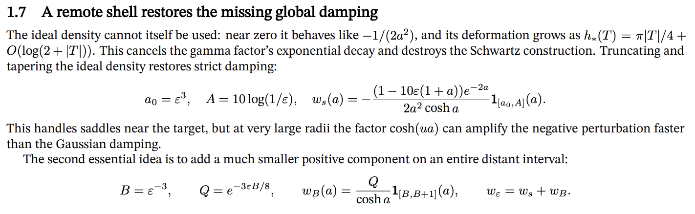
reasoning-walkthroughs.pdf.
I have no idea how these PDFs were written, but obviously, the difference suggests that they were not written by humans. Fortunately, the choice is not important for the final result, and the original choice is also valid—see the later section on reformalization.
The next three definitions give exactly the perturbed Gamma factor $E_\lambda(t) := E_\lambda^G(t) \exp(\lambda h(t/\lambda))$ and the Mellin transforms $X_+$, $X_-$.
-- Eλ(t) = π^(it/2) Γ((λ − it)/2) exp(λh(t/λ)).
def saddleEnvelope (ε ℓ t : ℝ) : ℂ :=
  Complex.exp
      (Complex.I * (t : ℂ) * (Real.log Real.pi : ℂ) / 2) *
    Complex.Gamma (((ℓ : ℂ) - Complex.I * (t : ℂ)) / 2) *
    Complex.exp ((ℓ : ℂ) *
      mellinShellPhase ε ((t : ℂ) / (ℓ : ℂ)))

-- X₊(t) = Eλ(t)P₊(t/λ).
def plusSaddleSpectrum (ε ℓ t : ℝ) : ℂ :=
  saddleEnvelope ε ℓ t *
    plusPolynomial ε ((t : ℂ) / (ℓ : ℂ))

-- X₋(t) = Eλ(t)P₋(t/λ).
def minusSaddleSpectrum (ε ℓ t : ℝ) : ℂ :=
  saddleEnvelope ε ℓ t *
    minusPolynomial ε ((t : ℂ) / (ℓ : ℂ))
For contour integration, the formal proof uses the usual variable $z=\lambda-it$. Thus $t/\lambda=i(z-\lambda)/\lambda$, and the Gamma factor becomes $\Gamma(z/2)$. The following definitions express the same functions in this coordinate; plusSaddleMellinData_vertical checks the correspondence explicitly. There is an analogous theorem for the minus sign.
-- Eλ in the coordinate z = λ − it.
def saddleMellinEnvelope (ε ℓ : ℝ) (z : ℂ) : ℂ :=
  Complex.exp
      (((ℓ : ℂ) - z) * (Real.log Real.pi : ℂ) / 2) *
    Complex.Gamma (z / 2) *
    Complex.exp ((ℓ : ℂ) *
      mellinShellPhase ε
        (Complex.I * (z - (ℓ : ℂ)) / (ℓ : ℂ)))

-- M₊(z) = Eλ(i(z − λ))P₊(i(z − λ)/λ).
def plusSaddleMellinData (ε ℓ : ℝ) (z : ℂ) : ℂ :=
  saddleMellinEnvelope ε ℓ z *
    plusPolynomial ε
      (Complex.I * (z - (ℓ : ℂ)) / (ℓ : ℂ))

-- M₊(λ − it) = X₊(t).
theorem plusSaddleMellinData_vertical (ε ℓ t : ℝ) :
    plusSaddleMellinData ε ℓ
      ((ℓ : ℂ) - Complex.I * (t : ℂ)) =
        plusSaddleSpectrum ε ℓ t := by ...
The radial profiles $f_\pm(r)$ are inverse Mellin transforms away from zero. Their common value at zero is defined as saddleOriginValue, whose agreement with the smooth extension is justified in the Smoothness and Values at the origin subsections below. The functions on $\mathbb R^d$ are obtained by substituting $r=\lVert x\rVert$.
-- f₊(r): inverse Mellin transform for r ≠ 0, prescribed value at r = 0.
def plusSaddleProfile (ε ℓ r : ℝ) : ℂ :=
  if r = 0 then (saddleOriginValue ε ℓ : ℂ)
  else mellinInv ℓ (plusSaddleMellinData ε ℓ) r

-- x ↦ f₊(‖x‖), with λ = d/2.
def plusSaddleFunction (ε : ℝ) (d : ℕ) (x : Euclidean d) : ℂ :=
  plusSaddleProfile ε ((d : ℝ) / 2) ‖x‖
To see the normalization hidden in mellinInv, one can use the next identity. It parametrizes the upward vertical line by $z=\lambda+it$, so $\mathrm{d}z=i\,\mathrm{d}t$ cancels the $i$ in $1/(2\pi i)$. Replacing $t$ by $-t$ recovers the inverse-transform formula in the overview.
-- The inverse-Mellin factor r⁻ᶻ.
def saddleMellinInversePower (r : ℝ) (z : ℂ) : ℂ :=
  (r : ℂ) ^ (-z)

-- f₊(r) = (1/2π) ∫ r^(−λ−it) M₊(λ + it) dt, for r > 0.
theorem plusSaddleProfile_eq_normalized_vertical_integral
    {ε ℓ r : ℝ} (hr : 0 < r) :
    plusSaddleProfile ε ℓ r =
      ((1 / (2 * Real.pi) : ℝ) : ℂ) *
        (∫ t : ℝ,
          saddleMellinInversePower r
            ((ℓ : ℂ) + (t : ℂ) * Complex.I) *
            plusSaddleMellinData ε ℓ
              ((ℓ : ℂ) + (t : ℂ) * Complex.I)) := by ...
Rapid decay at infinity
In the $t$-coordinate, we move the contour upward from $\Im t=0$ to an arbitrary positive height $\Im t=a-\lambda$, with $a>\lambda$. In the new coordinate $z=\lambda-it$, this corresponds to moving the contour from $\Re z=\lambda$ to $\Re z=a$. No poles are crossed, and $|r^{-z}|=r^{-a}$ on the new line. Taking $a$ arbitrarily large gives decay faster than every inverse power of $r$.
The following statements give the integrability and contour-shift identity for $f_+$. Their $f_-$ counterparts have the same names with plus replaced by minus. The condition hpole excludes the Gamma poles; it holds automatically when $a>0$.
-- Every polynomial moment of M₊(a + it) is integrable away from pole lines.
theorem plusSaddleMellinData_shiftedLine_moment_integrable
    {ε ℓ a : ℝ} (hε : 0 < ε) (hℓ : 0 < ℓ)
    (horder : shortCutoff ε ≤ shortEndpoint ε)
    (hpole : ∀ n : ℕ, a ≠ -((2 * n : ℕ) : ℝ))
    (j : ℕ) :
    Integrable (fun t : ℝ =>
      (t : ℂ) ^ j * plusSaddleMellinData ε ℓ
        ((a : ℂ) + (t : ℂ) * Complex.I)) := by ...

-- The inverse Mellin contour can be placed on any line Re z = a > 0.
theorem plusSaddleProfile_eq_positive_contour
    {ε ℓ r a : ℝ}
    (hε : 0 < ε) (hℓ : 0 < ℓ)
    (horder : shortCutoff ε ≤ shortEndpoint ε)
    (hr : 0 < r) (ha : 0 < a) :
    plusSaddleProfile ε ℓ r =
      ((1 / (2 * Real.pi) : ℝ) : ℂ) *
        (∫ t : ℝ,
          saddleMellinInversePower r
              ((a : ℂ) + (t : ℂ) * Complex.I) *
            plusSaddleMellinData ε ℓ
              ((a : ℂ) + (t : ℂ) * Complex.I)) := by ...
The contour identity uses plusSaddleMellinData_positive_vertical_integral_eq: apply Cauchy’s theorem to a rectangle in the right half-plane, then let its height tend to infinity. The horizontal integrals tend to zero.
For derivatives, Lean works with the squared radius $u=r^2$; this u is not the saddle ordinate. For $u>1$, the integral saddlePositiveContourMoment a j D u is the $j$-th derivative of $\int u^{-(a+it)/2}D(t)\,\mathrm dt$. Differentiation contributes a degree-$j$ polynomial in $t$, whose integrability follows from the moment bound above.
-- The shifted inverse Mellin integral, written as a function of u = r².
def plusSaddlePositiveSquaredContour
    (ε ℓ a u : ℝ) : ℂ :=
  ((1 / (2 * Real.pi) : ℝ) : ℂ) *
    saddlePositiveContourMoment a 0
      (fun t : ℝ =>
        plusSaddleMellinData ε ℓ
          ((a : ℂ) + (t : ℂ) * Complex.I)) u

-- Recover f₊ by substituting u = r².
theorem plusSaddleProfile_eq_positive_squaredContour
    {ε ℓ r a : ℝ}
    (hε : 0 < ε) (hℓ : 0 < ℓ)
    (horder : shortCutoff ε ≤ shortEndpoint ε)
    (hr : 0 < r) (ha : 0 < a) :
    plusSaddleProfile ε ℓ r =
      plusSaddlePositiveSquaredContour ε ℓ a (r ^ 2) := by ...
The estimate saddlePositiveContourMoment_norm_le bounds the $j$-th derivative by $C_{a,j}u^{-a/2-j}$. To bound it after multiplication by $u^k$, Lean takes $a=2(k+1)$. It also inserts a smooth cutoff, equal to zero for $u\le2$ and one for $u\ge3$, to separate the tail from the origin argument.
-- A smooth cutoff: 0 for u ≤ 2, and 1 for u ≥ 3.
def saddleOuterCutoff (u : ℝ) : ℂ :=
  (Real.smoothTransition (u - 2) : ℂ)

-- The outer parts agree with f₊(√u) for u ≥ 3.
def plusSaddleOuterSquaredProfile (ε ℓ u : ℝ) : ℂ :=
  saddleOuterCutoff u *
    plusSaddlePositiveSquaredContour ε ℓ 2 u

-- Every derivative of the outer plus profile decays faster than any power.
theorem plusSaddleOuterSquaredProfile_schwartz_decay
    {ε ℓ : ℝ}
    (hε : 0 < ε) (hℓ : 0 < ℓ)
    (horder : shortCutoff ε ≤ shortEndpoint ε)
    (k n : ℕ) :
    ∃ C : ℝ, ∀ u : ℝ,
      ‖u‖ ^ k *
        ‖iteratedFDeriv ℝ n
          (plusSaddleOuterSquaredProfile ε ℓ) u‖ ≤ C := by ...
Although the outer profiles are defined using the line $a=2$, contour independence lets the proof choose a larger $a$ for each decay estimate. Finally, saddleSquaredSchwartzPullback substitutes $u=\lVert x\rVert^2$ to obtain Schwartz tails on $\mathbb R^d$. Once smoothness at the origin is proved, the difference between each function and its tail is smooth and compactly supported, completing Schwartz regularity.
Smoothness
To study smoothness at the origin, shift the contour to the left past finitely many Gamma poles. First, factor the Mellin data as $\Gamma(z/2)$ times a holomorphic factor. The residues at $z=-2n$ are then $2(-1)^n/n!$ times that factor.
-- The common Mellin factor without Γ(z/2).
def saddleRegularMellinFactor (ε ℓ : ℝ) (z : ℂ) : ℂ :=
  Complex.exp
      (((ℓ : ℂ) - z) * (Real.log Real.pi : ℂ) / 2) *
    Complex.exp ((ℓ : ℂ) *
      mellinShellPhase ε
        (Complex.I * (z - (ℓ : ℂ)) / (ℓ : ℂ)))

-- M₊(z) = Γ(z/2) times this holomorphic factor and the polynomial P₊.
def plusSaddleRegularMellinFactor (ε ℓ : ℝ) (z : ℂ) : ℂ :=
  saddleRegularMellinFactor ε ℓ z *
    plusPolynomial ε
      (Complex.I * (z - (ℓ : ℂ)) / (ℓ : ℂ))

-- Residue of M₊ at z = −2n.
def plusSaddlePoleResidue (ε ℓ : ℝ) (n : ℕ) : ℂ :=
  (2 : ℂ) * (-1 : ℂ) ^ n / (n.factorial : ℂ) *
    plusSaddleRegularMellinFactor ε ℓ
      (-((2 * n : ℕ) : ℂ))
We shift the Mellin contour to $\Re z=-(2N+1)$, between the poles $-2N$ and $-2(N+1)$. The next definition is the remaining contour integral before dividing by $f_+(0)$.
-- The shifted line has Re z = −(2N + 1).
def saddleTaylorContour (N : ℕ) : ℝ :=
  -((2 * N + 1 : ℕ) : ℝ)

-- The unnormalized contour remainder after crossing N + 1 poles.
def plusSaddleTaylorRemainder
    (ε ℓ : ℝ) (N : ℕ) (r : ℝ) : ℂ :=
  ((1 / (2 * Real.pi) : ℝ) : ℂ) *
    (∫ t : ℝ,
      saddleMellinInversePower r
        ((saddleTaylorContour N : ℂ) +
          (t : ℂ) * Complex.I) *
        plusSaddleMellinData ε ℓ
          ((saddleTaylorContour N : ℂ) +
            (t : ℂ) * Complex.I))
The identity below makes the connection with the radial function. It expresses the function as a polynomial in $r^2$ plus a remainder term. The $n=0$ term is evaluated in the “Values at the origin” subsection below. The minus version is minusSaddleProfile_eq_residue_sum_add_remainder.
-- f₊(r) = Σₙ₌₀ᴺ Resₙ r²ⁿ + contour remainder.
theorem plusSaddleProfile_eq_residue_sum_add_remainder
    {ε ℓ r : ℝ}
    (hε : 0 < ε) (hℓ : 0 < ℓ)
    (horder : shortCutoff ε ≤ shortEndpoint ε)
    (hr : 0 < r) (N : ℕ) :
    plusSaddleProfile ε ℓ r =
      (∑ n ∈ Finset.range (N + 1),
        plusSaddlePoleResidue ε ℓ n *
          ((r ^ (2 * n) : ℝ) : ℂ)) +
      plusSaddleTaylorRemainder ε ℓ N r := by ...
The residue expansion and the bounds on its differentiated remainders prove smoothness at the origin; away from zero, one differentiates the inverse Mellin integral. The formal proof carries out the origin argument in $u = r^2$, so the conclusion is smoothness of the functions on $\mathbb R^d$, not just of their radial profiles:
-- The radial function f₊ is C∞, including at x = 0.
theorem plusSaddleFunction_contDiff
    {ε : ℝ} (hε : 0 < ε)
    {d : ℕ} (hd : 0 < d)
    (horder : shortCutoff ε ≤ shortEndpoint ε) :
    ContDiff ℝ ∞ (plusSaddleFunction ε d) := by ...
Values at the origin
The real-valued function $u\mapsto h(iu)$ is defined as realHyperbolicShellPhase. Since $h$ is even, its value at $u=1$ is also $h(-i)$. This explains the formula for saddleOriginValue.
-- h(iu) = ∫ w(a)(cosh(au) − 1) da, as a real number.
def realHyperbolicShellPhase (ε u : ℝ) : ℝ :=
  (∫ a in shortCutoff ε..shortEndpoint ε,
    shortShellDensity ε a * (Real.cosh (a * u) - 1)) +
  (∫ a in shellLocation ε..shellLocation ε + 1,
    positiveShellDensity ε a * (Real.cosh (a * u) - 1))

-- The complex phase at iu equals its real hyperbolic expression.
theorem mellinShellPhase_imaginary (ε u : ℝ) :
    mellinShellPhase ε (Complex.I * (u : ℂ)) =
      (realHyperbolicShellPhase ε u : ℂ) := by ...

-- f₊(0) = f₋(0) = 2π^(λ/2) exp(λh(−i))β.
def saddleOriginValue (ε ℓ : ℝ) : ℝ :=
  2 * Real.pi ^ (ℓ / 2) *
    Real.exp (ℓ * realHyperbolicShellPhase ε 1) * beta ε

-- The common origin value is positive when ε > 0.
theorem saddleOriginValue_pos {ε : ℝ} (hε : 0 < ε) (ℓ : ℝ) :
    0 < saddleOriginValue ε ℓ := by ...

-- P₊(−i) = β.
theorem plusPolynomial_neg_I (ε : ℝ) :
    plusPolynomial ε (-Complex.I) = (beta ε : ℂ) := by ...

-- P₋(−i) = β.
theorem minusPolynomial_neg_I (ε : ℝ) :
    minusPolynomial ε (-Complex.I) = (beta ε : ℂ) := by ...
The first residue, at $z=0$, agrees with the prescribed common value:
-- The residue at z = 0 equals to f₊(0).
theorem plusSaddlePoleResidue_zero
    {ε ℓ : ℝ} (hℓ : 0 < ℓ) :
    plusSaddlePoleResidue ε ℓ 0 =
      (saddleOriginValue ε ℓ : ℂ) := by ...

-- The residue at z = 0 equals to f₋(0).
theorem minusSaddlePoleResidue_zero
    {ε ℓ : ℝ} (hℓ : 0 < ℓ) :
    minusSaddlePoleResidue ε ℓ 0 =
      (saddleOriginValue ε ℓ : ℂ) := by ...
Finally, the following simplification lemmas evaluate the defined functions at zero. Together with the smoothness proved above and the first-residue computation, this identifies the value of the continuous extension of the inverse Mellin integral.
-- The defined f₊ takes the common origin value at x = 0.
@[simp] theorem plusSaddleFunction_zero (ε : ℝ) (d : ℕ) :
    plusSaddleFunction ε d (0 : Euclidean d) =
      (saddleOriginValue ε ((d : ℝ) / 2) : ℂ) := by ...

-- The defined f₋ takes the same origin value at x = 0.
@[simp] theorem minusSaddleFunction_zero (ε : ℝ) (d : ℕ) :
    minusSaddleFunction ε d (0 : Euclidean d) =
      (saddleOriginValue ε ((d : ℝ) / 2) : ℂ) := by ...
Realness, Schwartzness, and the Fourier identity
These functions are also real-valued.
-- Im f₊(x) = 0.
theorem plusSaddleFunction_real (ε : ℝ) (d : ℕ)
    (x : Euclidean d) :
    (plusSaddleFunction ε d x).im = 0 := by ...

-- Im f₋(x) = 0.
theorem minusSaddleFunction_real (ε : ℝ) (d : ℕ)
    (x : Euclidean d) :
    (minusSaddleFunction ε d x).im = 0 := by ...
Combining smoothness with rapid decay, plusSaddleSchwartz packages $f_+$ as a Schwartz function on $\mathbb R^d$.
We also have minusSaddleSchwartz for $f_-$. Radiality follows from the definitions through $\lVert x\rVert$.
def plusSaddleSchwartz
    {ε : ℝ} (hε : 0 < ε)
    {d : ℕ} (hd : 0 < d)
    (horder : shortCutoff ε ≤ shortEndpoint ε) :
    TestFunction d where ...
Finally, saddleSource_fourier_minus_eq_plus proves that the Fourier transform of fminus is fplus.
-- Fourier(f₋) = f₊.
theorem saddleSource_fourier_minus_eq_plus
    {ε : ℝ} (hε : 0 < ε) {d : ℕ} (hd : 0 < d)
    (horder : shortCutoff ε ≤ shortEndpoint ε)
    (fminus fplus : TestFunction d)
    (hminus : ∀ x : Euclidean d,
      fminus x = minusSaddleFunction ε d x)
    (hplus : ∀ x : Euclidean d,
      fplus x = plusSaddleFunction ε d x) :
    (𝓕 fminus : TestFunction d) = fplus := by ...
Sign analysis
First, here are the logarithmic radius $v(u)$ and the two radius thresholds. The integral terms in saddleLogRadius equal $ih^{\prime}(iu)$. Notice that the parameter ε in saddleSmallRadiusStarOrdinate is unused mathematically: $u_\ast$ depends only on $d$.
Note that the complex digamma function is in mathlib, but not the real one.
For some reason, there’s also saddleSourceStationaryLogRadius, which is essentially the same as saddleLogRadius with $\lambda = d/2$.
I don’t know why there are two of them.
-- ψ(x) = (log Γ)′(x).
def saddleDigamma (x : ℝ) : ℝ :=
  deriv (Real.log ∘ Real.Gamma) x

-- v(u) = −½ log π + ½ψ(λ(1 + u)/2) + ih′(iu).
def saddleLogRadius (ε : ℝ) (d : ℕ) (u : ℝ) : ℝ :=
  -(Real.log Real.pi) / 2 +
    saddleDigamma (((d : ℝ) / 2) * (1 + u) / 2) / 2 +
    (∫ a in shortCutoff ε..shortEndpoint ε,
      shortShellDensity ε a * a * Real.sinh (u * a)) +
    (∫ a in shellLocation ε..shellLocation ε + 1,
      positiveShellDensity ε a * a * Real.sinh (u * a))

-- u★ = −1 + log λ/(4λ).
def saddleSmallRadiusStarOrdinate (ε : ℝ) (d : ℕ) : ℝ :=
  let _sourceParameter : ℝ := ε
  show ℝ from
    -1 + Real.log ((d : ℝ) / 2) /
      (4 * ((d : ℝ) / 2))

-- r★ = exp(v(u★)).
def saddleSmallRadiusStar (ε : ℝ) (d : ℕ) : ℝ :=
  Real.exp
    (saddleLogRadius ε d
      (saddleSmallRadiusStarOrdinate ε d))

-- Rε,d = exp(v(1 + ε/4)).
def saddleSourceRadius (ε : ℝ) (d : ℕ) : ℝ :=
  Real.exp (saddleLogRadius ε d (1 + ε / 4))
The shifted integral. The contour $t=\lambda(T+iu)$ becomes $z=\lambda(1+u)-i\lambda T$. Lean divides the Mellin factor on this contour by the positive number $E_\lambda(i\lambda u)$, then multiplies by $e^{i\lambda Tv}$. At $v=v(u)$, saddleSourceCenteredEnvelope is precisely $e^{\mathcal L_u(T)}$.
-- z(T) = λ(1 + u) − iλT.
def saddleSourceMellinContour (ℓ u T : ℝ) : ℂ :=
  ((ℓ * (1 + u) : ℝ) : ℂ) -
    Complex.I * ((ℓ * T : ℝ) : ℂ)

-- Eλ(iλu), a positive real number for λ > 0 and u > −1.
def saddleSourceContourEnvelopeScale
    (ε ℓ u : ℝ) : ℝ :=
  Real.exp (-(ℓ * u) * Real.log Real.pi / 2) *
    Real.Gamma (ℓ * (1 + u) / 2) *
      Real.exp (ℓ * realHyperbolicShellPhase ε u)

-- Eλ(λ(T + iu))/Eλ(iλu).
def saddleSourceNormalizedEnvelope
    (ε ℓ u T : ℝ) : ℂ :=
  saddleMellinEnvelope ε ℓ
      (saddleSourceMellinContour ℓ u T) /
    (saddleSourceContourEnvelopeScale ε ℓ u : ℂ)

-- The normalized factor multiplied by exp(iλTv).
def saddleSourceCenteredEnvelope
    (ε ℓ u v T : ℝ) : ℂ :=
  saddleSourceNormalizedEnvelope ε ℓ u T *
    Complex.exp (Complex.I * ((ℓ * T * v : ℝ) : ℂ))

-- At v = v(u): exp(ℒᵤ(T))P₊(T + iu).
def saddleSourceCenteredPlusIntegrand
    (ε ℓ u v T : ℝ) : ℂ :=
  saddleSourceCenteredEnvelope ε ℓ u v T *
    plusPolynomial ε ((T : ℂ) + Complex.I * (u : ℂ))

-- At v = v(u): exp(ℒᵤ(T))P₋(T + iu).
def saddleSourceCenteredMinusIntegrand
    (ε ℓ u v T : ℝ) : ℂ :=
  saddleSourceCenteredEnvelope ε ℓ u v T *
    minusPolynomial ε ((T : ℂ) + Complex.I * (u : ℂ))

-- The real prefactor λEλ(iλu) exp(−λ(1 + u)v)/(2π).
def saddleSourceCenteredPrefactor
    (ε ℓ u v : ℝ) : ℝ :=
  (ℓ / (2 * Real.pi)) *
    Real.exp (-(ℓ * (1 + u) * v)) *
      saddleSourceContourEnvelopeScale ε ℓ u

-- The prefactor is positive for λ > 0 and u > −1.
theorem saddleSourceCenteredPrefactor_pos
    {ε ℓ u : ℝ} (hℓ : 0 < ℓ) (hu : -1 < u)
    (v : ℝ) :
    0 < saddleSourceCenteredPrefactor ε ℓ u v := by ...

-- f₊(exp v) = positive prefactor × centered integral.
theorem plusSaddleProfile_exp_eq_centeredIntegral
    {ε ℓ u : ℝ}
    (hε : 0 < ε) (hℓ : 0 < ℓ) (hu : -1 < u)
    (horder : shortCutoff ε ≤ shortEndpoint ε)
    (v : ℝ) :
    plusSaddleProfile ε ℓ (Real.exp v) =
      (saddleSourceCenteredPrefactor ε ℓ u v : ℂ) *
        (∫ T : ℝ,
          saddleSourceCenteredPlusIntegrand ε ℓ u v T) := by ...
The analogous identity for $f_-$ is minusSaddleProfile_exp_eq_centeredIntegral. Both identities hold for any real $v$; only later is $v$ chosen to make $T=0$ stationary.
The Gaussian approximation. The variance is assembled from the Gamma contribution and the signed weight contribution. Here δ = u - 1, so 2 + δ = 1 + u. These quantities give the same $V(u)=v^{\prime}(u)$ as in Part 1.
-- The Gamma contribution: λ⁻¹ ∫ a² μλ,u(a) da, with u = η − 1.
def upperGammaVariance (ℓ η : ℝ) : ℝ :=
  ℓ⁻¹ * ∫ a : ℝ in Set.Ioi 0,
    a ^ 2 * upperGammaMeasureDensity ℓ η a

-- The positive-weight variance minus the negative-weight magnitude.
def upperNetShellVariance (ε δ : ℝ) : ℝ :=
  upperPositiveShellVariance ε δ -
    upperShortShellVariance ε δ

-- V(1 + δ) = Gamma variance + signed weight variance.
def upperSaddleVariance (ε ℓ δ : ℝ) : ℝ :=
  upperGammaVariance ℓ (2 + δ) +
    upperNetShellVariance ε δ

-- V(u), obtained by substituting δ = u − 1.
def saddleSourceGaussianVariance
    (ε ℓ u : ℝ) : ℝ :=
  upperSaddleVariance ε ℓ (u - 1)

-- Gᵤ(T) = exp(−λV(u)T²/2).
def saddleSourceGaussianKernel
    (ε ℓ u T : ℝ) : ℝ :=
  Real.exp
    (-(ℓ * saddleSourceGaussianVariance ε ℓ u / 2) * T ^ 2)

-- Gᵤ(T)P₊(iu).
def saddleSourceGaussianPlusIntegrand
    (ε ℓ u T : ℝ) : ℂ :=
  (saddleSourceGaussianKernel ε ℓ u T : ℂ) *
    plusPolynomial ε (Complex.I * (u : ℂ))

-- Gᵤ(T)P₋(iu).
def saddleSourceGaussianMinusIntegrand
    (ε ℓ u T : ℝ) : ℂ :=
  (saddleSourceGaussianKernel ε ℓ u T : ℂ) *
    minusPolynomial ε (Complex.I * (u : ℂ))

-- For λ > 0 and V(u) > 0, ∫ Gᵤ(T) dT = √(2π/(λV(u))).
theorem saddleSourceGaussianKernel_integral
    (ε ℓ u : ℝ) :
    (∫ T : ℝ, saddleSourceGaussianKernel ε ℓ u T) =
      Real.sqrt
        (Real.pi /
          (ℓ * saddleSourceGaussianVariance ε ℓ u / 2)) := by ...

-- T★ = (λ(1 + u))^(1/12)/√(λV(u)).
def saddleSourceFirstBranchCentralRadius
    (ε ℓ u : ℝ) : ℝ :=
  (ℓ * (1 + u)) ^ (1 / 12 : ℝ) /
    Real.sqrt (ℓ * saddleSourceGaussianVariance ε ℓ u)

-- T★ = λ^(1/12)/√(λV(u)).
def saddleSourceSecondBranchCentralRadius
    (ε ℓ u : ℝ) : ℝ :=
  ℓ ^ (1 / 12 : ℝ) /
    Real.sqrt (ℓ * saddleSourceGaussianVariance ε ℓ u)
The variance positivity is proved in eventually_saddleSourceGaussianVariance_firstBranch_pos and eventually_saddleSourceGaussianVariance_secondBranch_pos. The following two theorems then give the full-line error bounds used for the signs.
For the first range, the condition $\log\lambda/4\le\lambda(1+u)$ is exactly $u\ge u_\ast$. The extra hypothesis for the minus sign is $u\ge u_0=1+\varepsilon/4$.
-- For u★ ≤ u ≤ U, the total Gaussian error is smaller than the main term.
theorem eventually_saddleSourceFirstBranch_fullGaussianErrors :
    ∀ᶠ ε : ℝ in 𝓝[>] (0 : ℝ),
      ∀ᶠ ℓ : ℝ in atTop,
        ∀ u : ℝ, -1 < u → u ≤ 1 + ε / 2 →
          Real.log ℓ / 4 ≤ ℓ * (1 + u) →
            (‖(∫ T : ℝ,
                saddleSourceCenteredPlusIntegrand ε ℓ u
                  (saddleSourceStationaryLogRadius ε ℓ u) T) -
              (∫ T : ℝ,
                saddleSourceGaussianPlusIntegrand ε ℓ u T)‖ <
              ‖plusPolynomial ε (Complex.I * (u : ℂ))‖ *
                (∫ T : ℝ,
                  saddleSourceGaussianKernel ε ℓ u T)) ∧
            (1 + ε / 4 ≤ u →
              ‖(∫ T : ℝ,
                  saddleSourceCenteredMinusIntegrand ε ℓ u
                    (saddleSourceStationaryLogRadius ε ℓ u) T) -
                (∫ T : ℝ,
                  saddleSourceGaussianMinusIntegrand ε ℓ u T)‖ <
                ‖minusPolynomial ε (Complex.I * (u : ℂ))‖ *
                  (∫ T : ℝ,
                    saddleSourceGaussianKernel ε ℓ u T)) := by ...
For the second range, the theorem uses $\delta=u-1$, so its condition $\delta\ge\varepsilon/2$ means $u\ge U$.
-- For u ≥ U, both Gaussian errors are smaller than their main terms.
theorem eventually_saddleSourceSecondBranch_fullGaussianErrors :
    ∀ᶠ ε : ℝ in 𝓝[>] (0 : ℝ),
      ∀ᶠ ℓ : ℝ in atTop,
        ∀ δ : ℝ, ε / 2 ≤ δ →
          (‖(∫ T : ℝ,
              saddleSourceCenteredPlusIntegrand ε ℓ (1 + δ)
                (saddleSourceStationaryLogRadius
                  ε ℓ (1 + δ)) T) -
            (∫ T : ℝ,
              saddleSourceGaussianPlusIntegrand ε ℓ (1 + δ) T)‖ <
            ‖plusPolynomial ε
              (Complex.I * ((1 + δ : ℝ) : ℂ))‖ *
              (∫ T : ℝ,
                saddleSourceGaussianKernel ε ℓ (1 + δ) T)) ∧
          (‖(∫ T : ℝ,
              saddleSourceCenteredMinusIntegrand ε ℓ (1 + δ)
                (saddleSourceStationaryLogRadius
                  ε ℓ (1 + δ)) T) -
            (∫ T : ℝ,
              saddleSourceGaussianMinusIntegrand ε ℓ (1 + δ) T)‖ <
            ‖minusPolynomial ε
              (Complex.I * ((1 + δ : ℝ) : ℂ))‖ *
              (∫ T : ℝ,
                saddleSourceGaussianKernel ε ℓ (1 + δ) T)) := by ...
Since the quantifiers ∀ᶠ ε in 𝓝[>] 0 and ∀ᶠ ℓ in atTop come before ∀ u or ∀ δ, the threshold is uniform over the indicated range. Substituting $\lambda=d/2$ gives the eventual dimension statements.
Each proof combines three estimates: the error on the central interval, the tail of the original integrand, and the Gaussian tail. For example, the first range uses eventually_saddleSourceFirstBranch_centralGaussianErrors, eventually_saddleSourceFirstBranch_sourceL1Tails, and eventually_saddleSourceFirstBranch_gaussianL1Tails. The second range has the corresponding SecondBranch lemmas. This is the same splitting as in Part 1; the final statements retain the strict inequality needed for signs rather than the full relative asymptotic.
From an integral estimate to a sign. The polynomial signs are elementary:
-- P₊(iu) > 0 for ε > 0 and u > −1.
theorem plusPolynomial_imaginary_re_pos {ε u : ℝ}
    (hε : 0 < ε) (hu : -1 < u) :
    0 < (plusPolynomial ε (Complex.I * (u : ℂ))).re := by ...

-- P₋(iu) < 0 for ε > 0 and u ≥ 1 + ε/4.
theorem minusPolynomial_imaginary_re_neg {ε u : ℝ}
    (hε : 0 < ε) (hu : 1 + ε / 4 ≤ u) :
    (minusPolynomial ε (Complex.I * (u : ℂ))).re < 0 := by ...
The next two theorems isolate the last step. If the complex error is smaller than the magnitude of the real Gaussian main term, its real part cannot change the sign. Multiplication by the positive prefactor preserves that sign.
-- A Gaussian error smaller than the positive main term gives f₊(exp v) > 0.
theorem plusSaddleProfile_exp_re_pos_of_gaussian_error
    {ε ℓ u v : ℝ}
    (hε : 0 < ε)
    (hℓ : 0 < ℓ)
    (hu : -1 < u)
    (horder : shortCutoff ε ≤ shortEndpoint ε)
    (hV : 0 < saddleSourceGaussianVariance ε ℓ u)
    (herror :
      ‖(∫ T : ℝ,
          saddleSourceCenteredPlusIntegrand ε ℓ u v T) -
        (∫ T : ℝ,
          saddleSourceGaussianPlusIntegrand ε ℓ u T)‖ <
        (∫ T : ℝ,
          saddleSourceGaussianPlusIntegrand ε ℓ u T).re) :
    0 < (plusSaddleProfile ε ℓ (Real.exp v)).re := by ...

-- A Gaussian error smaller than the negative main term's magnitude gives f₋(exp v) < 0.
theorem minusSaddleProfile_exp_re_neg_of_gaussian_error
    {ε ℓ u v : ℝ}
    (hε : 0 < ε)
    (hℓ : 0 < ℓ)
    (hu : -1 < u)
    (horder : shortCutoff ε ≤ shortEndpoint ε)
    (hV : 0 < saddleSourceGaussianVariance ε ℓ u)
    (herror :
      ‖(∫ T : ℝ,
          saddleSourceCenteredMinusIntegrand ε ℓ u v T) -
        (∫ T : ℝ,
          saddleSourceGaussianMinusIntegrand ε ℓ u T)‖ <
        -(∫ T : ℝ,
          saddleSourceGaussianMinusIntegrand ε ℓ u T).re) :
    (minusSaddleProfile ε ℓ (Real.exp v)).re < 0 := by ...
Finally, estimates at radii $e^{v(u)}$ must cover all the radii we need. Lean proves this using continuity of $v$ and $v(u)\to\infty$, followed by the intermediate value theorem; strict monotonicity is not required for this particular step.
-- Every r ≥ r★ equals exp(v(u)) for some u ≥ u★.
theorem eventually_saddleSmallRadiusStar_log_coverage :
    ∀ᶠ ε : ℝ in 𝓝[>] (0 : ℝ),
      ∀ᶠ d : ℕ in atTop,
        ∀ r : ℝ,
          saddleSmallRadiusStar ε d ≤ r →
            ∃ u : ℝ,
              saddleSmallRadiusStarOrdinate ε d ≤ u ∧
                saddleLogRadius ε d u = Real.log r := by ...

-- Every r ≥ Rε,d equals exp(v(u)) for some u ≥ u₀.
theorem eventually_saddleSourceRadius_log_coverage :
    ∀ᶠ ε : ℝ in 𝓝[>] (0 : ℝ),
      ∀ d : ℕ, 0 < d →
        ∀ r : ℝ,
          saddleSourceRadius ε d ≤ r →
            ∃ u : ℝ,
              1 + ε / 4 ≤ u ∧
                saddleLogRadius ε d u = Real.log r := by ...
Combining these with the sign estimates proves $f_+(r)>0$ for $r\ge r_\ast$ and $f_-(r)<0$ for $r\ge R_{\varepsilon,d}$. Only the interval $0\le r\le r_\ast$ for $f_+$ remains.
Positivity of $f_+$ for small radii
Here are the scaled variable $y$ and the coefficients $A_{\lambda,n}$ in the residue expansion. The quantity saddleShellDerivativeOne is $ih^{\prime}(i)=\int w(a)a\sinh(a)\,da$.
-- h₁′ = ih′(i) = ∫ w(a)a sinh(a) da.
def saddleShellDerivativeOne (ε : ℝ) : ℝ :=
  (∫ a in shortCutoff ε..shortEndpoint ε,
    shortShellDensity ε a * a * Real.sinh a) +
  (∫ a in shellLocation ε..shellLocation ε + 1,
    positiveShellDensity ε a * a * Real.sinh a)

-- y = πr² exp(2h₁′).
def saddleSmallRadiusVariable (ε r : ℝ) : ℝ :=
  Real.pi * Real.exp (2 * saddleShellDerivativeOne ε) * r ^ 2

-- Aλ,n: the normalized coefficient of (−y)ⁿ/n! in the residue sum.
def plusSaddleSmallRadiusCoefficient
    (ε ℓ : ℝ) (n : ℕ) : ℝ :=
  Real.exp
      (ℓ *
        (realHyperbolicShellPhase ε
          (1 + 2 * (n : ℝ) / ℓ) -
            realHyperbolicShellPhase ε 1) -
        2 * (n : ℝ) * saddleShellDerivativeOne ε) *
    ((beta ε - (2 * (n : ℝ) / ℓ) *
        (2 + 2 * (n : ℝ) / ℓ) ^ 2) /
      beta ε)
Using the contour remainder defined in the Smoothness subsection, Lean rewrites the residue expansion in terms of $y$ and divides by the common origin value:
-- f₊(r)/f₊(0) = Σₙ₌₀ᴺ (−y)ⁿAλ,n/n! + normalized remainder.
theorem plusSaddleProfile_div_origin_eq_small_radius_residue_series
    {ε ℓ r : ℝ}
    (hε : 0 < ε) (hℓ : 0 < ℓ)
    (horder : shortCutoff ε ≤ shortEndpoint ε)
    (hr : 0 < r) (N : ℕ) :
    plusSaddleProfile ε ℓ r /
        (saddleOriginValue ε ℓ : ℂ) =
      ((∑ n ∈ Finset.range (N + 1),
        (-saddleSmallRadiusVariable ε r) ^ n /
          (n.factorial : ℝ) *
            plusSaddleSmallRadiusCoefficient ε ℓ n : ℝ) : ℂ) +
      plusSaddleTaylorRemainder ε ℓ N r /
        (saddleOriginValue ε ℓ : ℂ) := by ...
Thus the plusSaddleTaylorRemainder in the code is not itself $\mathcal R_\lambda$ from the overview: it must be divided by saddleOriginValue.
The coefficient estimate below is a quantitative version of $A_{\lambda,n}=1+O_\varepsilon(n(1+n)/\lambda)$. Its exponential factor is harmless when $n\le N$ and $N^2/\lambda\to0$.
-- Bound |Aλ,n − 1| by C(n + n²)exp(Cn²/λ)/λ, for 2n ≤ λ.
theorem exists_plusSaddleSmallRadiusCoefficient_error
    {ε : ℝ}
    (hε : 0 < ε)
    (horder : shortCutoff ε ≤ shortEndpoint ε) :
    ∃ C : ℝ, 0 ≤ C ∧
      ∀ (ℓ : ℝ), 0 < ℓ →
        ∀ n : ℕ, 2 * (n : ℝ) ≤ ℓ →
          |plusSaddleSmallRadiusCoefficient ε ℓ n - 1| ≤
            (C * ((n : ℝ) + (n : ℝ) ^ 2) / ℓ) *
              Real.exp (C * (n : ℝ) ^ 2 / ℓ) := by ...

-- N = ⌈20 log λ⌉.
def saddleSmallResidueTruncation (ℓ : ℝ) : ℕ :=
  Nat.ceil (20 * Real.log ℓ)

-- Uniformly for 0 ≤ r ≤ r★, y ≤ (log λ)/8 + Cε.
theorem exists_eventually_y_star_le_log_eighth_add
    {ε : ℝ} (hε : 0 < ε)
    (horder : shortCutoff ε ≤ shortEndpoint ε) :
    ∃ C : ℝ, 0 ≤ C ∧
      ∀ᶠ d : ℕ in atTop,
        ∀ r : ℝ, 0 ≤ r →
          r ≤ saddleSmallRadiusStar ε d →
            saddleSmallRadiusVariable ε r ≤
              Real.log ((d : ℝ) / 2) / 8 + C := by ...
The finite residue sum has two errors: its coefficients $A_{\lambda,n}$ differ from $1$, and the exponential series is truncated. The first theorem below controls their combined error; the second controls the contour remainder. Both bounds are relative errors, obtained after multiplying by $e^y$.
-- Uniformly on 0 ≤ r ≤ r★, eʸ|S_N(y) − e⁻ʸ| < 1/2.
theorem eventually_plusSaddleSmallRadius_relativeFiniteResidue_lt_half_on_star
    {ε : ℝ}
    (hε : 0 < ε)
    (horder : shortCutoff ε ≤ shortEndpoint ε) :
    ∀ᶠ d : ℕ in atTop,
      ∀ r : ℝ,
        0 ≤ r → r ≤ saddleSmallRadiusStar ε d →
          let ℓ : ℝ := (d : ℝ) / 2
          let y : ℝ := saddleSmallRadiusVariable ε r
          Real.exp y *
            |(∑ n ∈ Finset.range
                (saddleSmallResidueTruncation ℓ + 1),
              ((-y) ^ n / (n.factorial : ℝ)) *
                plusSaddleSmallRadiusCoefficient ε ℓ n) -
              Real.exp (-y)| < 1 / 2 := by ...

-- Uniformly on 0 < r ≤ r★, eʸ|normalized remainder| < 1/2.
theorem eventually_plusSaddleTaylorRemainder_relative_lt_half_on_star
    {ε : ℝ}
    (hε : 0 < ε) (hεsmall : ε ≤ 1 / 4)
    (horder : shortCutoff ε ≤ shortEndpoint ε)
    (hmargin : ∀ a ∈ Icc (shortCutoff ε) (shortEndpoint ε),
      0 ≤ shortMargin ε a) :
    ∀ᶠ d : ℕ in atTop,
      ∀ r : ℝ, 0 < r → r ≤ saddleSmallRadiusStar ε d →
        let ℓ : ℝ := (d : ℝ) / 2
        let N : ℕ := saddleSmallResidueTruncation ℓ
        let y : ℝ := saddleSmallRadiusVariable ε r
        Real.exp y *
          ‖plusSaddleTaylorRemainder ε ℓ N r /
            (saddleOriginValue ε ℓ : ℂ)‖ < 1 / 2 := by ...
The first bound allows $r=0$; the contour bound is stated only for $r>0$. The extra hmargin assumption says that $b(a)\ge0$ on the short interval, so the designated negative weight really is nonpositive. All these parameter conditions hold for sufficiently small positive $\varepsilon$.
The final implication is now elementary: the finite sum is greater than $e^{-y}/2$, while the real part of the normalized remainder is greater than $-e^{-y}/2$. Their sum is positive.
-- The two strict relative errors below 1/2 imply f₊(r) > 0.
theorem plusSaddleProfile_re_pos_of_relative_residue_bounds
    {ε ℓ r : ℝ}
    (hε : 0 < ε)
    (hℓ : 0 < ℓ)
    (horder : shortCutoff ε ≤ shortEndpoint ε)
    (hr : 0 < r)
    (N : ℕ)
    (hfinite :
      Real.exp (saddleSmallRadiusVariable ε r) *
        |(∑ n ∈ Finset.range (N + 1),
            (-saddleSmallRadiusVariable ε r) ^ n /
              (n.factorial : ℝ) *
                plusSaddleSmallRadiusCoefficient ε ℓ n) -
          Real.exp (-(saddleSmallRadiusVariable ε r))| <
        (1 / 2 : ℝ))
    (hremainder :
      Real.exp (saddleSmallRadiusVariable ε r) *
        ‖plusSaddleTaylorRemainder ε ℓ N r /
          (saddleOriginValue ε ℓ : ℂ)‖ <
        (1 / 2 : ℝ)) :
    0 < (plusSaddleProfile ε ℓ r).re := by ...

-- For small ε and large d, f₊(r) > 0 throughout 0 ≤ r ≤ r★.
theorem eventually_plusSaddleProfile_re_pos_on_star :
    ∀ᶠ ε : ℝ in 𝓝[>] (0 : ℝ),
      ∀ᶠ d : ℕ in atTop,
        ∀ r : ℝ, 0 ≤ r → r ≤ saddleSmallRadiusStar ε d →
          0 < (plusSaddleProfile ε ((d : ℝ) / 2) r).re := by ...
The last theorem handles $r=0$ using saddleOriginValue_pos.
Combining this with the critical point argument completes the signs required by the LP construction.
-- For small ε and large d: f₊ ≥ 0 everywhere, and f₋ ≤ 0 for ‖x‖ ≥ Rε,d.
def SaddleSourceEventualSigns : Prop :=
  ∀ᶠ ε : ℝ in 𝓝[>] (0 : ℝ),
    ∀ᶠ d : ℕ in atTop,
      (∀ x : Euclidean d,
        0 ≤ (plusSaddleFunction ε d x).re) ∧
      (∀ x : Euclidean d,
        saddleSourceRadius ε d ≤ ‖x‖ →
          (minusSaddleFunction ε d x).re ≤ 0)

theorem saddleSourceEventualSigns : SaddleSourceEventualSigns := by ...
Radius asymptotics and the LP upper bound
The Fourier identity, common positive origin value, and sign conditions now give the functions needed for the LP construction. As in the last step of the proof summary, the digamma asymptotic and the weight integrals give
\[\frac{R_{\varepsilon,d}}{\sqrt d}\longrightarrow\alpha_\varepsilon \quad(d\to\infty), \qquad \alpha_\varepsilon\longrightarrow\frac1\pi \quad(\varepsilon\to0^+).\]Here $\alpha_\varepsilon$ is limitingSaddleRadius ε.
-- αε = √((1 + u₀)/(4π)) exp(∫ w(a)a sinh(u₀a) da).
def limitingSaddleRadius (ε : ℝ) : ℝ :=
  Real.sqrt ((2 + ε / 4) / (4 * Real.pi)) *
    Real.exp (shortShellRadiusContribution ε +
      positiveShellRadiusContribution ε)

-- For fixed ε > 0, Rε,d/√d → αε as d → ∞.
theorem tendsto_saddleSourceRadius_normalized
    {ε : ℝ} (hε : 0 < ε) :
    Tendsto
      (fun d : ℕ =>
        saddleSourceRadius ε d / Real.sqrt (d : ℝ))
      atTop (𝓝 (limitingSaddleRadius ε)) := by ...

-- αε → 1/π as ε → 0⁺.
theorem tendsto_limitingSaddleRadius :
    Tendsto limitingSaddleRadius (𝓝[>] (0 : ℝ))
      (nhds criticalRadius) := by ...
The first limit uses tendsto_saddleDigamma_sub_log, which says $\psi(x)-\log x\to0$. For the second, the contribution of $w_s$ tends to $-\frac12\log(\pi/2)$, while the contribution of $w_B$ tends to zero; these are tendsto_shortShellRadiusContribution, integral_wallisRadiusIntegrand, and tendsto_positiveShellRadiusContribution.
Rescaling by $F(x)=f_-(R_{\varepsilon,d}x)$ makes the exterior sign condition hold for $\lVert x\rVert\ge1$. Fourier scaling and the equal origin values then give
\[\frac{F(0)}{\widehat F(0)}=R_{\varepsilon,d}^{\,d}, \qquad \mathrm{LP}_d^{1/d}\le\frac{v_d^{1/d}}2R_{\varepsilon,d}.\]The constructor saddleSourceAdmissible performs this rescaling. The next theorem computes its quotient; saddleSourceAdmissible_normalizedCost then takes the $d$-th root and divides by $\sqrt d$, giving exactly $R/\sqrt d$.
-- The rescaled admissible function has F(0)/F̂(0) = Rᵈ.
theorem saddleSourceAdmissible_quotient
    {ε : ℝ} (hε : 0 < ε) {d : ℕ} (hd : 0 < d)
    (horder : shortCutoff ε ≤ shortEndpoint ε)
    {R : ℝ} (hR : 0 < R)
    (fminus fplus : TestFunction d)
    (hminus : ∀ x : Euclidean d,
      fminus x = minusSaddleFunction ε d x)
    (hplus : ∀ x : Euclidean d,
      fplus x = plusSaddleFunction ε d x)
    (hplusnonneg : ∀ x : Euclidean d,
      0 ≤ (plusSaddleFunction ε d x).re)
    (hminusoutside : ∀ x : Euclidean d,
      R ≤ ‖x‖ → (minusSaddleFunction ε d x).re ≤ 0) :
    quotient (saddleSourceAdmissible hε hd horder hR
      fminus fplus hminus hplus hplusnonneg
      hminusoutside) = R ^ d := by ...

-- The normalized objective is the d-th root of the quotient, divided by √d.
def normalizedCost {d : ℕ} (f : Admissible d) : ℝ :=
  quotient f ^ ((d : ℝ)⁻¹) / Real.sqrt (d : ℝ)

-- Take the infimum over admissible functions.
def normalizedProgram (d : ℕ) : ℝ :=
  sInf (Set.range (normalizedCost (d := d)))
The two radius limits and the admissible functions are combined into OrderedEpsilonUpperConstruction.
-- Record the limits in d and ε, together with eventual admissible witnesses.
structure OrderedEpsilonUpperConstruction where
  epsilonBound : ℝ
  epsilonBound_pos : 0 < epsilonBound
  normalizedRadius : ℝ → ℕ → ℝ
  limitingRadius : ℝ → ℝ
  limitingRadius_tendsto :
    Tendsto limitingRadius (𝓝[>] (0 : ℝ)) (𝓝 criticalRadius)
  normalizedRadius_tendsto :
    ∀ ε : ℝ, 0 < ε → ε < epsilonBound →
      Tendsto (normalizedRadius ε) atTop (𝓝 (limitingRadius ε))
  admissibleWitness :
    ∀ ε : ℝ, 0 < ε → ε < epsilonBound →
      ∀ᶠ d : ℕ in atTop,
        ∃ f : Admissible d, normalizedCost f ≤ normalizedRadius ε d

-- Assemble this data from the Schwartz functions and their sign estimates.
noncomputable def saddleOrderedUpperConstruction_of_sourceSigns
    (hsigns : SaddleSourceEventualSigns) :
    OrderedEpsilonUpperConstruction :=
  saddleOrderedUpperConstruction
    saddleSourceSchwartzRealization hsigns

-- Every c > 1/π eventually bounds the normalized cost of some admissible f.
def ConstructivePrimalUpperBound : Prop :=
  ∀ c : ℝ, criticalRadius < c →
    ∀ᶠ d : ℕ in atTop,
      ∃ f : Admissible d, normalizedCost f ≤ c

theorem constructivePrimal_of_orderedEpsilon
    (construction : OrderedEpsilonUpperConstruction) :
    ConstructivePrimalUpperBound := by ...
The last proof fixes $c>1/\pi$, chooses a sufficiently small $\varepsilon$ with $\alpha_\varepsilon<c$, and then takes $d$ large enough that $R_{\varepsilon,d}/\sqrt d<c$ and the sign conditions hold. Thus the required dimension may depend on $\varepsilon$.
Using $v_d^{1/d}\sqrt d\to\sqrt{2\pi e}$, first let $d\to\infty$ and then $\varepsilon\to0^+$. This gives the upper bound $\limsup_{d\to\infty}\mathrm{LP}_d^{1/d}\le\sqrt{e/(2\pi)}$, completing the argument.
In Lean, the upper bound is first combined with the lower bound to prove normalizedProgram d → 1/π. The geometric factor then converts this to the limit of $\mathrm{LP}_d^{1/d}$.
-- The normalized LP objective tends to 1/π.
def SharpQuotientAsymptotic : Prop :=
  Tendsto normalizedProgram atTop (nhds criticalRadius)

theorem sharpQuotient_of_uniform_lower_and_ordered_upper
    (hlower : UniformAdmissibleLowerBound)
    (construction : OrderedEpsilonUpperConstruction) :
    SharpQuotientAsymptotic := by ...

-- The geometric factor is v_d^(1/d) √d / 2, for d > 0.
def packingGeometricRoot (d : ℕ) : ℝ :=
  (unitBallVolume d / (2 : ℝ) ^ d) ^ ((d : ℝ)⁻¹) *
    Real.sqrt (d : ℝ)

-- LP_d^(1/d) = geometric factor × normalized objective.
theorem linearProgram_root_eq_geometric_mul_normalizedProgram_unconditional
    {d : ℕ} (hd : 0 < d) :
    (linearProgram d) ^ ((d : ℝ)⁻¹) =
      packingGeometricRoot d * normalizedProgram d := by ...

-- Stirling's formula gives the geometric limit √(2πe)/2.
theorem tendsto_packingGeometricRoot :
    Tendsto packingGeometricRoot atTop
      (nhds (Real.sqrt (2 * Real.pi * Real.exp 1) / 2)) := by ...

def criticalPackingBase : ℝ :=
  Real.sqrt (Real.exp 1 / (2 * Real.pi))

-- The final limit is LP_d^(1/d) → √(e/(2π)).
def SharpPackingRootAsymptotic : Prop :=
  Tendsto (fun d : ℕ => (linearProgram d) ^ ((d : ℝ)⁻¹))
    atTop (nhds criticalPackingBase)

theorem sharpPackingRoot_of_sharpQuotient
    (hquotient : SharpQuotientAsymptotic) :
    SharpPackingRootAsymptotic := by ...

theorem sharpPackingRootAsymptotic : SharpPackingRootAsymptotic :=
  sharpAsymptotics.2.1
Reformalization
After checking the original proof and the formalization, I decided to refactor the formalization. There were several goals for this:
- Make it more readable, with comments and a blueprint.
- Make it more modular and complete.
- Figure out if the change of parameter choices in the formalization is necessary, or if the original choices are sufficient.
- Formalize missing results.
- Figure out which parts can be upstreamed to mathlib.
- Keep the default
maxHeartbeatsunchanged.
The result can be found here.
The refactoring was done by Claude (orchestrated by Fable 5.1 until I reached the usage limit) with a Max (x20) subscription. I used to have x5, but I decided to upgrade to x20 for this project.
I started by writing RefactoringPlan.md myself, and simply asked Claude to follow it.
It uses the original report, the original formalization, and drafts of the blog posts (this post and Part 1).
I also added further guidance while refactoring, after I realized that the initial plan was incomplete.
As a result, the refactored formalization is almost half the size of the original formalization if you put everything into a single file (see SpherePackingRefactored.lean).
You should not compare it directly with the original formalization, since it proves more results but also removes some unnecessary results (I could also make it shorter by removing all the comments, but I haven’t).
I also asked Claude to record important changes in RefactoringResult.md, which is complete slop but contains notable updates.
The main differences are:
-
Both the $(+1)$ and $(-1)$ sign-uncertainty principles are formalized in terms of $L^1$ (integrable) functions, not only Schwartz functions. In particular, the reduction from $L^1$ to Schwartz functions is formalized, which is not in the original formalization.
structure SignEigenfunction (d : ℕ) (ς : ℤˣ) where toFun : Euclidean d → ℝ integrable : Integrable toFun fourier_eq : ∀ ξ : Euclidean d, 𝓕 (fun x ↦ (toFun x : ℂ)) ξ = ((ς : ℤ) : ℂ) * toFun ξ ne_zero : toFun ≠ 0 zero : toFun 0 = 0 theorem exists_schwartz_approximation (hd : 0 < d) (h : SignEigenfunction d ς) (hrad : IsRadial h) : ∃ q : ℕ → TestFunction d, (∀ n, IsRealValued (q n) ∧ IsRadial (q n) ∧ (𝓕 (q n) : TestFunction d) = ((ς : ℤ) : ℂ) • q n ∧ q n 0 = 0) ∧ Tendsto (fun n ↦ ∫ x, ‖q n x - (h x : ℂ)‖) atTop (𝓝 0) := by ... -
Radial reduction is formalized for both problems; in particular, the refactored formalization includes the radial reduction for the $L^1$ sign-uncertainty problem. Radialization averages a function over the orthogonal group.
LP_eq_radialandsignUncertaintyConstant_eq_radialstate the two reductions. HereAdmissibleabbreviatesPackingBounds.FullAdmissible.variable {E : Type*} [NormedAddCommGroup E] [NormedSpace ℝ E] def rotationalAverage (g : Euclidean d → E) (x : Euclidean d) : E := ∫ U : OrthogonalGroup d, g (orthogonalAction U⁻¹ x) ∂radialOrthogonalHaar d structure FullAdmissible (d : ℕ) where function : CohnElkies.TestFunction d real : ∀ x : CohnElkies.Euclidean d, (function x).im = 0 fourier_real : ∀ x : CohnElkies.Euclidean d, ((𝓕 function) x).im = 0 fourier_nonneg : ∀ x : CohnElkies.Euclidean d, 0 ≤ ((𝓕 function) x).re fourier_zero_pos : 0 < ((𝓕 function) (0 : CohnElkies.Euclidean d)).re outside_nonpos : ∀ x : CohnElkies.Euclidean d, 1 ≤ ‖x‖ → (function x).re ≤ 0 structure RadialAdmissible (d : ℕ) extends toAdmissible : Admissible d where /-- The function is radial. -/ radial : IsRadial function def Admissible.radialize {d : ℕ} (f : Admissible d) : RadialAdmissible d := ... theorem LP_eq_radial (d : ℕ) : LP d = unitBallVolume d / 2 ^ d * sInf (Set.range fun f : RadialAdmissible d ↦ quotient f.toAdmissible) := ... theorem signUncertaintyConstant_eq_radial (hd : 0 < d) (ς : ℤˣ) : signUncertaintyConstant ς d = ⨅ (g : SignEigenfunction d ς) (_ : IsRadial (g : Euclidean d → ℝ)), signRadius g := by ... -
The refactored formalization uses the original parameter choices, showing that they suffice for the argument. The parameter names have also been changed to make them more consistent with the report.
def a₀ε (ε : ℝ) : ℝ := ε ^ 2 def Aε (ε : ℝ) : ℝ := log (1 / ε) def Bε (ε : ℝ) : ℝ := ε⁻¹ ^ 3 def Qε (ε : ℝ) : ℝ := exp (-3 * ε * Bε ε / 8) def bε (ε a : ℝ) : ℝ := 1 - 2 * ε * (1 + a) def β (ε : ℝ) : ℝ := ε / 4 -
(Updated 2026.09.20) Proposition A.1 is also formalized, showing $\mathsf{A}_+(d) < \mathsf{A}_-(d)$ for all $d\ge1$. The operator $T_d$ is defined in
TailIntegral.lean:def tailIntegral (d : ℕ) (g : Euclidean d → ℝ) (x : Euclidean d) : ℝ := if x = 0 then 0 else (d / 2 : ℝ) / 2 * ∫ t in Ioi (1 : ℝ), t ^ ((d / 2 : ℝ) - 1) * g (t • x)As in the report, the vanishing central Mellin moment gives a second formula integrating over $(0,1)$. This proves continuity at the origin; Tonelli gives the $L^1$ bound, and Fourier scaling gives the $(+1)$-eigenfunction property. Strict positivity at and beyond $r(g)$, followed by continuity, gives the smaller sign radius in
AppendixA.lean.namespace SignEigenfunction variable (hd : 0 < d) (g : SignEigenfunction d (-1)) (hg : IsRadial (g : Euclidean d → ℝ)) include hd hg -- ‖T_d g‖₁ ≤ ½ ‖g‖₁. theorem integral_norm_tailIntegral_le : ∫ x, ‖tailIntegral d g x‖ ≤ 1 / 2 * ∫ x, ‖g x‖ := by ... -- A finite last-sign radius strictly decreases. theorem signRadius_tailIntegral_lt (hfin : signRadius (g : Euclidean d → ℝ) < ⊤) : signRadius (tailIntegral d g) < signRadius g := by ... end SignEigenfunction -- Package T_d g as a nonzero, integrable (+1)-eigenfunction vanishing at 0. def SignEigenfunction.tailIntegral (hd : 0 < d) (g : SignEigenfunction d (-1)) (hg : IsRadial (g : Euclidean d → ℝ)) : SignEigenfunction d 1 where toFun := _root_.CohnElkies.tailIntegral d g integrable := g.integrable_tailIntegral hd hg fourier_eq ξ := by rw [g.fourier_tailIntegral hd hg ξ] simp ne_zero := g.tailIntegral_ne_zero hd hg zero := tailIntegral_zero _To obtain a strict inequality between the infima, we also need an extremizer for $\mathsf{A}_-(d)$, whose existence is established in Theorem 1.4 of Cohn–Gonçalves (2019), §3.2. Both proofs take a weak $L^2$ limit of an $L^1$-normalized minimizing sequence. The main difference is how they prevent the limit from being zero: Cohn–Gonçalves use the Nazarov–Jaming uncertainty principle, while the formalization proves the following qualitative substitute by compactness in
EigenfunctionConcentration.lean.namespace Real variable {V : Type*} [NormedAddCommGroup V] [InnerProductSpace ℝ V] [FiniteDimensional ℝ V] [MeasurableSpace V] [BorelSpace V] -- A normalized Fourier eigenfunction has uniformly positive mass outside any fixed ball. theorem exists_pos_le_setIntegral_norm_compl_closedBall_of_fourier_eq_mul [Nontrivial V] {c : ℂ} (hc : c ≠ 0) (R : ℝ) : ∃ κ : ℝ, 0 < κ ∧ ∀ f : V → ℂ, Integrable f → (∀ ξ, 𝓕 f ξ = c * f ξ) → ∫ x, ‖f x‖ = 1 → κ ≤ ∫ x in (Metric.closedBall (0 : V) R)ᶜ, ‖f x‖ := by ... end RealOtherwise, a sequence concentrating inside the ball would give a nonzero, compactly supported limit whose Fourier transform is also compactly supported, contradicting Fourier analyticity. The formalization also avoids Mazur’s lemma: it passes the needed properties to the weak limit by testing against suitable $L^2$ functions, then applies the Gaussian correction from Cohn–Gonçalves’ Lemma 3.1 to make the value at the origin zero. Radializing the resulting extremizer and applying $T_d$ finishes the proof.
-- The infimum A₋(d) is attained.
theorem exists_signRadius_eq_signUncertaintyConstant_neg_one (hd : 0 < d) :
    ∃ g : SignEigenfunction d (-1),
      signRadius (g : Euclidean d → ℝ) = signUncertaintyConstant (-1) d := by ...

-- Apply T_d to a radial extremizer: A₊(d) ≤ r(T_d g) < r(g) = A₋(d).
theorem signUncertaintyConstant_one_lt_neg_one (hd : 0 < d) :
    signUncertaintyConstant 1 d < signUncertaintyConstant (-1) d := by ...
The additional assertion in Proposition A.1 that $T_d$ preserves Schwartz functions is not included in these lemmas; it is not needed for the $L^1$ sign-uncertainty comparison.
-
(Updated 2026.09.21) Added a proof of Lemma 3.2 that uses the Poisson inequality. In particular, we defined subharmonic functions and proved the Poisson inequality using Jensen’s identity (inequality).
A function is subharmonic on $U$ if it is upper semicontinuous, does not take the value $+\infty$, and satisfies the sub-mean-value inequality.
structure SubharmonicOn (u : ℂ → EReal) (U : Set ℂ) : Prop where
  /-- `u` is upper semicontinuous on `U`. -/
  upperSemicontinuousOn : UpperSemicontinuousOn u U
  /-- `u` does not take the value `⊤ = +∞` on `U`. -/
  ne_top : ∀ z ∈ U, u z ≠ ⊤
  /-- The sub-mean-value inequality: for every `z ∈ U`, all sufficiently small radii `r > 0` and
  every level `a : ℝ`, `u z` is at most the circle average of the truncation `(max u a).toReal`
  over the circle of radius `r` around `z`. -/
  le_circleAverage : ∀ z ∈ U, ∀ᶠ r in 𝓝[>] (0 : ℝ), ∀ a : ℝ,
    u z ≤ ((circleAverage (fun w ↦ EReal.truncateToReal a (u w)) z r : ℝ) : EReal)
When $f$ is a holomorphic function, $\log\lvert f\rvert$ is subharmonic. Also, subharmonic functions satisfy the maximum principle.
theorem AnalyticOnNhd.subharmonicOn_log_enorm {f : ℂ → ℂ} (hU : IsOpen U)
    (hf : AnalyticOnNhd ℂ f U) : SubharmonicOn (fun z ↦ ENNReal.log ‖f z‖ₑ) U := by ...

theorem le_zero_of_limsup_frontier {Ω : Set ℂ} (hΩ : IsOpen Ω) (hb : Bornology.IsBounded Ω)
    (hc : IsPreconnected Ω) (hu : SubharmonicOn u Ω)
    (hfr : ∀ ζ ∈ frontier Ω, limsup u (𝓝[Ω] ζ) ≤ 0) : ∀ z ∈ Ω, u z ≤ 0 := by ...
The following
le_poissonIntegralHalfPlanetheorem proves the Poisson inequality.noncomputable def poissonKernelHalfPlane (z : ℂ) (x : ℝ) : ℝ := π⁻¹ * z.im / ((x - z.re) ^ 2 + z.im ^ 2) noncomputable def poissonIntegralHalfPlane (b : ℝ → ℝ) (z : ℂ) : ℝ := ∫ x, poissonKernelHalfPlane z x * b x theorem le_poissonIntegralHalfPlane {b : ℝ → ℝ} {E : Finset ℝ} {M : ℝ} (hu : SubharmonicOn u {z | 0 < z.im}) (hM : ∀ z : ℂ, 0 < z.im → u z ≤ M) (hb : Integrable fun x ↦ b x / (1 + x ^ 2)) (hbc : ∀ x : ℝ, x ∉ E → ContinuousAt b x) (hbdry : ∀ x : ℝ, x ∉ E → limsup u (𝓝[{z | 0 < z.im}] (x : ℂ)) ≤ (b x : EReal)) : ∀ z : ℂ, 0 < z.im → u z ≤ (poissonIntegralHalfPlane b z : EReal) := by ... -
The
CohnElkiesForMathlibdirectory contains parts of the formalization that might be upstreamed to mathlib. Since these were all chosen by Claude, we cannot guarantee that they are indeed upstreamable. But after checking, I found that most of them are indeed useful. They include:fourier_comp_linearEquiv: if $g(x) = f(Ax)$ for an invertible linear map $A$, then $\hat g(\xi) = \frac{1}{\lvert\det A\rvert}\hat f(A^{-T}\xi)$.integrable_fourierIntegral_of_deriv_deriv: if $f:\mathbb R\to\mathbb C$ is twice differentiable and $f,f^{\prime},f^{\prime\prime}$ are integrable, then $\hat f$ is integrable.PhragmenLindelof.horizontal_strip_norm_extension: the Phragmén-Lindelöf principle for holomorphic functions whose norm extends continuously to the boundary of a horizontal strip, with the appropriate growth condition. This generalizesPhragmenLindelof.horizontal_stripin mathlib.Complex.tendsto_add_natCast_mul_Gamma_nhdsNE: residues of the Gamma function at all nonpositive integers. Mathlib already has the residue at zero asComplex.tendsto_self_mul_Gamma_nhds_zero, as well as the corresponding result for the completed Gamma factor,Complex.Gammaℝ_residue_zero.Real.digammaand its asymptotics: Mathlib only hasComplex.digamma. Also,tendsto_digamma_sub_log_atTopproves $\psi(x)-\log x\to0$ as $x\to\infty$.coth: Mathlib only hassinh,cosh, andtanh(but it hascot!).
-
The default
maxHeartbeatsis no longer changed. I guess the main reason for increasing it was the 30-digit approximation of the Cohn-Elkies exponent in the original formalization, which requires huge numerical certificates but is not important at all. So I simply removed it.
Conclusion
We went through OpenAI’s formalization of their result and found that it is incomplete. Someone may say that I’m too picky, since the main LP argument is formalized. But the report makes additional sign-uncertainty claims, and those deserve separate statements and proofs.
There are a lot of autoformalized results (and there will be more in the future) in which the formalized statement $A^{\prime}$ is not exactly the same as the natural-language statement $A$, but $A^{\prime}$ is just a few trivial steps away from $A$, so you might think this is fine. But if that is really the case, why don’t you just formalize $A$ directly? This is because, most of the time, people don’t read the AI’s autoformalized proofs and just believe them. This belief will make more sense as AI gets better and better, but then it will generate longer slop formalizations, and similar issues will persist. If you want to autoformalize a natural-language proof, the best thing you can do is to make every formal statement and argument as close to the natural-language proof as possible, using the same notation and no more or fewer lemmas. More importantly, make a blueprint. If your AI is good enough to autoformalize a natural-language proof, then it should be good enough to automatically write a blueprint that is not too bad for a human to read and understand (just push the button a few more times), which is way better than having no blueprint at all. I recently wrote a blog post about this on the Proofs and Prompts community blog (prompted by other news)—check it out here.
Let me end the series of posts with a question and answer:
Q. Does this proof give any further insight into these problems?
A.
¯\_(ツ)_/¯
Use of LLMs
Both ChatGPT and Claude were used to understand the formalization. My first prompt asked for a one-to-one correspondence between the informal statements and proofs in the report and the formal statements and proofs in Lean. Both LLMs spotted the same missing statements. As mentioned above, I used Claude to refactor the formalization.
Tags:math ai formalization